Animal parents often choose where to have their offspring in the place that will give them the best chance at success. They look for places that have plentiful food, low risk of predation, and good climate.
Even though parents pick out these spots, individuals often move away from their birthplace at some point in their lives. Why do animals move away? There are risks that come with moving from one place to another. It can be dangerous to go through unknown places – potentially stumbling into predators or being exposed to diseases. But there can also be benefits to moving, such as discovering a better spot to live as an adult, finding mates, and spreading out to reduce competition.
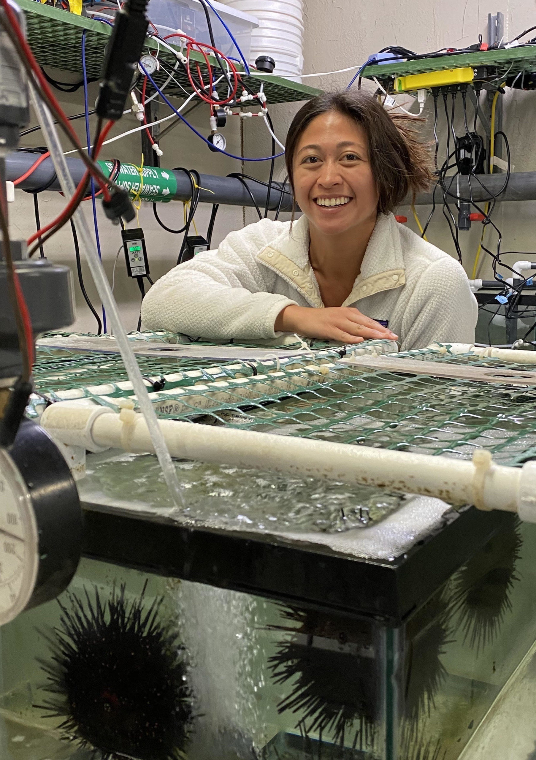
As someone who loves to travel and has lived in four different countries, Isabela can relate! Isabela likes to see new places, try new foods, and learn new languages. But there can be drawbacks, and occasionally she finds it hard to be in a completely new place. Sometimes people don’t understand her accent, or she can’t understand them. She also misses her family when she is away. Knowing that traveling and moving can have such highs and lows for herself, Isabela wanted to know more about what motivates animals to seek out new places.
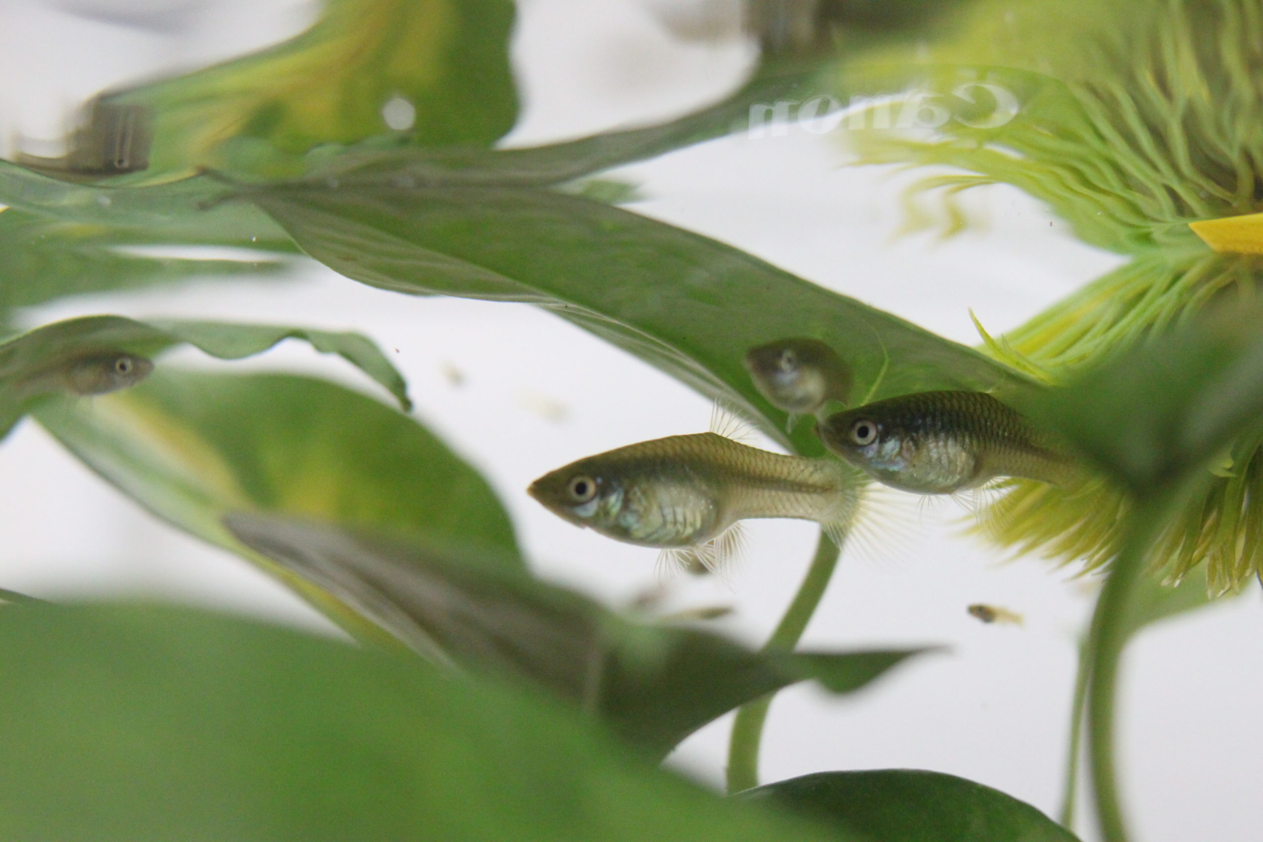
To follow her curiosity, Isabela found a graduate advisor who was also interested in animal movement. She joined Sarah’s lab because she had already collected data on the movement of small tropical fish called guppies. Sarah is part of a large collaborative project, where researchers from all over the world come together in Trinidad to study these fish populations.
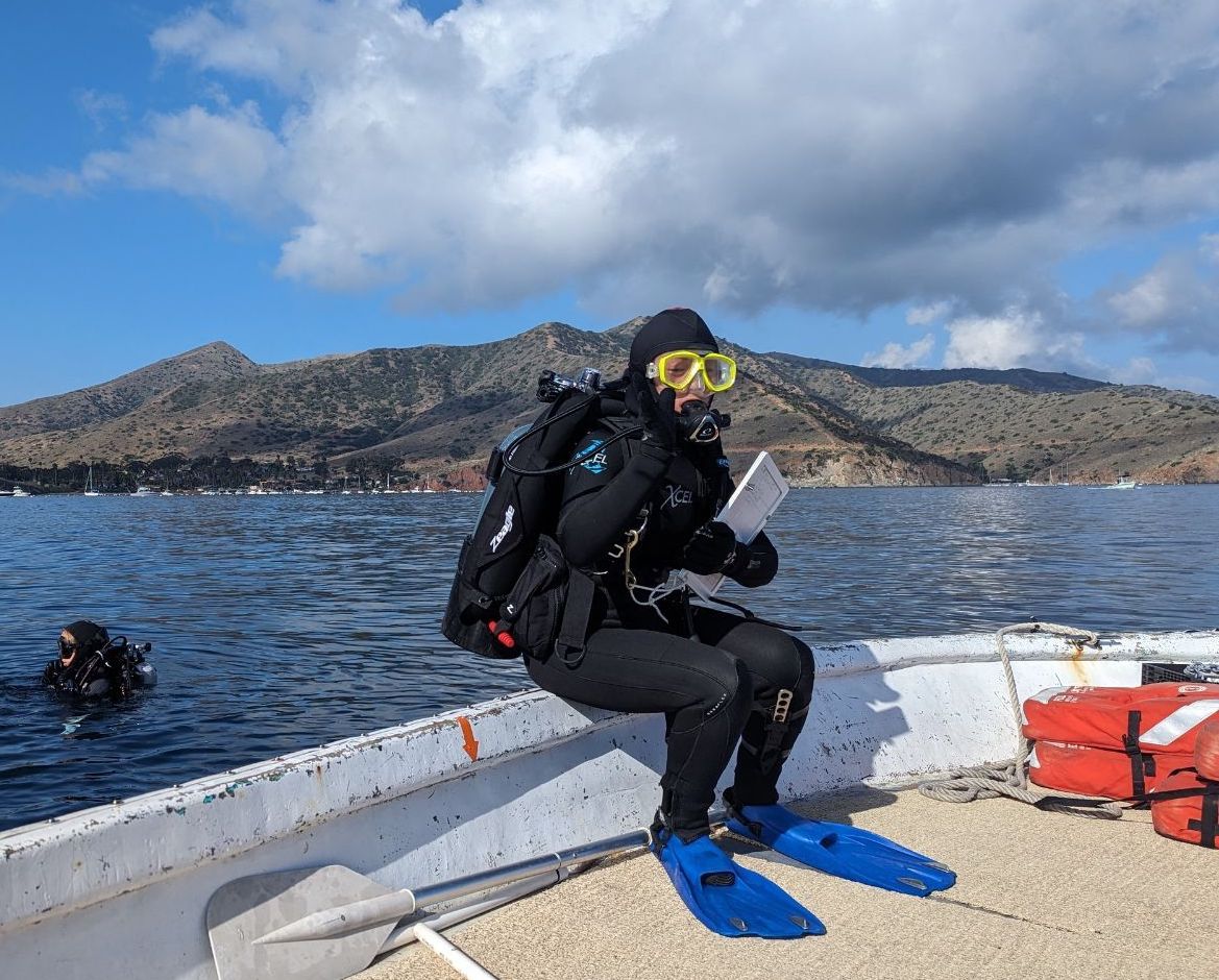
When Sarah first started collecting data in this system, she wanted to track how far guppies move from one place to the next. She used established protocols from previous work in this system to set up a study. With the help of a team, she captured every fish in two similar streams for replication. Every fish that was caught was marked with a small tattoo so the research team could recognize it if it was found again in the future. She did this same procedure every month for 14 months. Each time she sampled the fish, she recorded the individuals that she found and where they were found.
Isabela used this dataset to ask whether guppies benefit from moving from one place to another. In this study, she focused on one type of benefit: having a higher number of offspring. It is through reproduction that animals are able to pass on their genes, so the more offspring an individual fish has, the more successful it is.
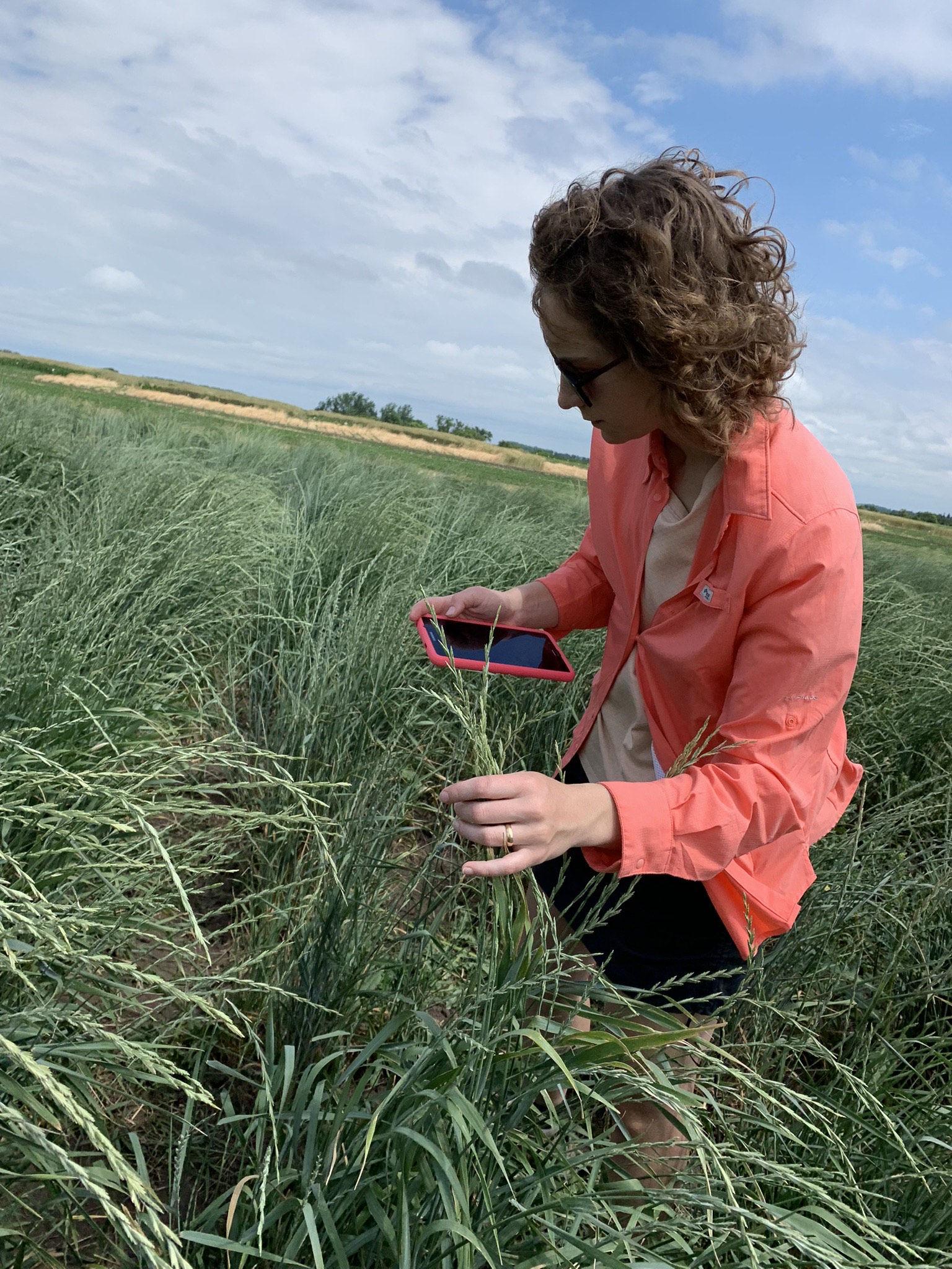
First, Isabela used the existing dataset to find out how far each fish moved: if Fish 1 was captured in Portion A of a stream in February and then in Portion B of the same stream in March, Isabela knew it had to move from A to B. She could use the timepoints to estimate how far each individual had traveled that month.
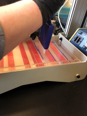
Second, Isabela used genetics to find out how many offspring each fish had. She looked at genetic markers to determine familial relationships between individuals in each stream. For example, two fish that shared 50% of their genes were probably a parent and an offspring. In this case, the older individual would be marked as the parent. Isabela used the genetic information to build a pedigree, or a chart that documents each generation of a population. That way she could track how many offspring each parent had produced.
She used these data to answer her question on whether there are benefits to traveling more. Isabela also wanted to compare whether the potential benefits of dispersal differed across the sexes. Males have to compete for females in order to mate. Isabela wanted to know if males that moved more were able to mate with more females and have more offspring.
Featured scientists: Isabela Borges (she/her) and Sarah Fitzpatrick (she/her) from the Kellogg Biological Station at Michigan State University.
Flesch–Kincaid Reading Grade Level = 8.3
Additional teacher resources related to this Data Nugget include:
If you or your students are interested in accessing more of the data behind this Data Nugget, you can download the full dataset from Isabella’s research and have students create graphs in Excel, Google Sheets, or using other data visualization software.
If students would like to learn more about Isabela, check out this Exploring with Scientists video from her time at the Kellogg Biological Station.
For more on this system and the research Sarah did in this study system, check out this unit and video on Galactic Polymath:
- Genetic Rescue to the Rescue (unit)
- Saving a species through genetic rescue: Why we need model organisms (video)