- Teacher Guide
- Student activity, Graph Type A, Level 3
- Student activity, Graph Type B, Level 3
- Student activity, Graph Type C, Level 3
- Grading Rubric
As you step into a warm greenhouse, you can feel how the glass has captured the sun’s heat inside. Now imagine that same warmth spreading across the entire planet due to increased greenhouse gas emissions. Climate scientists predict that by the year 2100, Earth’s average temperature could increase by as much as 3°C because of climate change. That might sound small, but even a few degrees matter a lot.
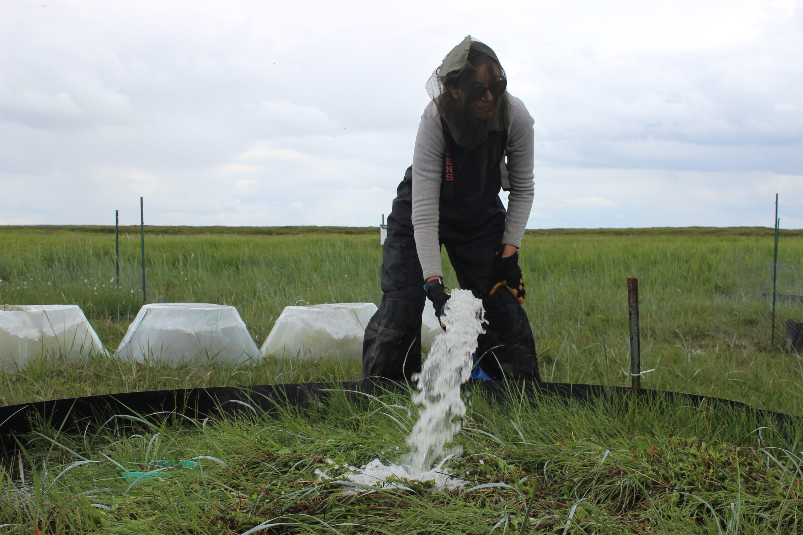
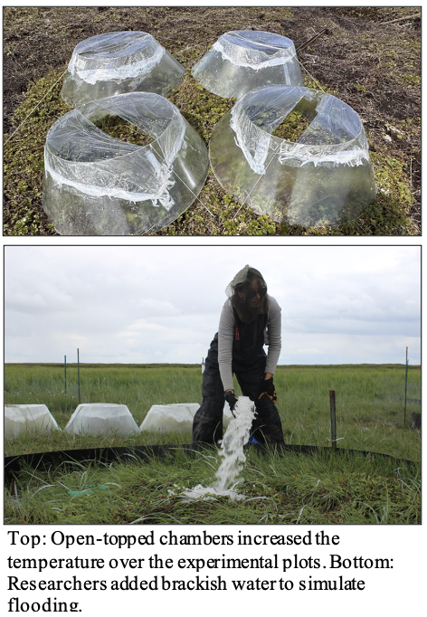
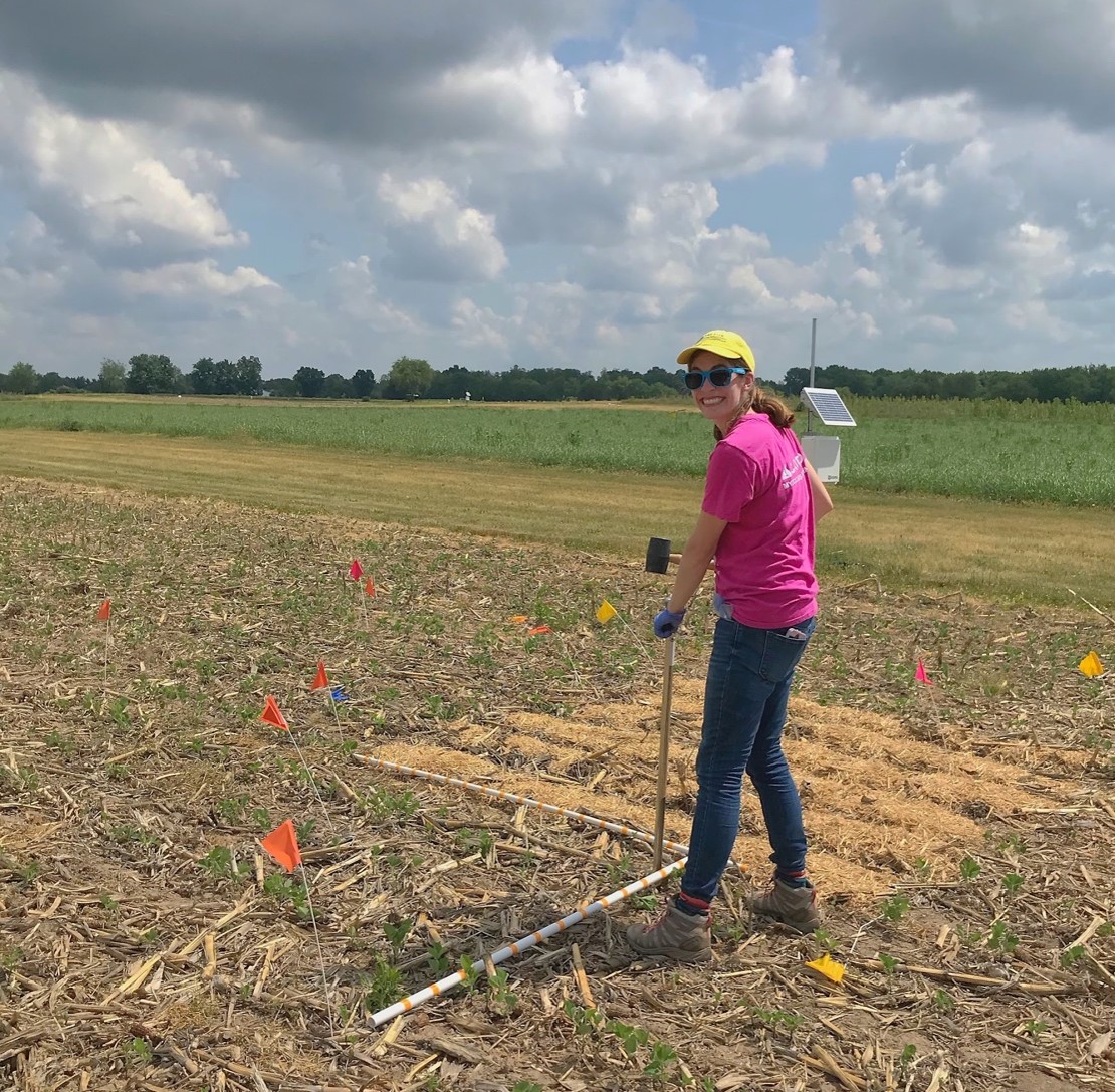
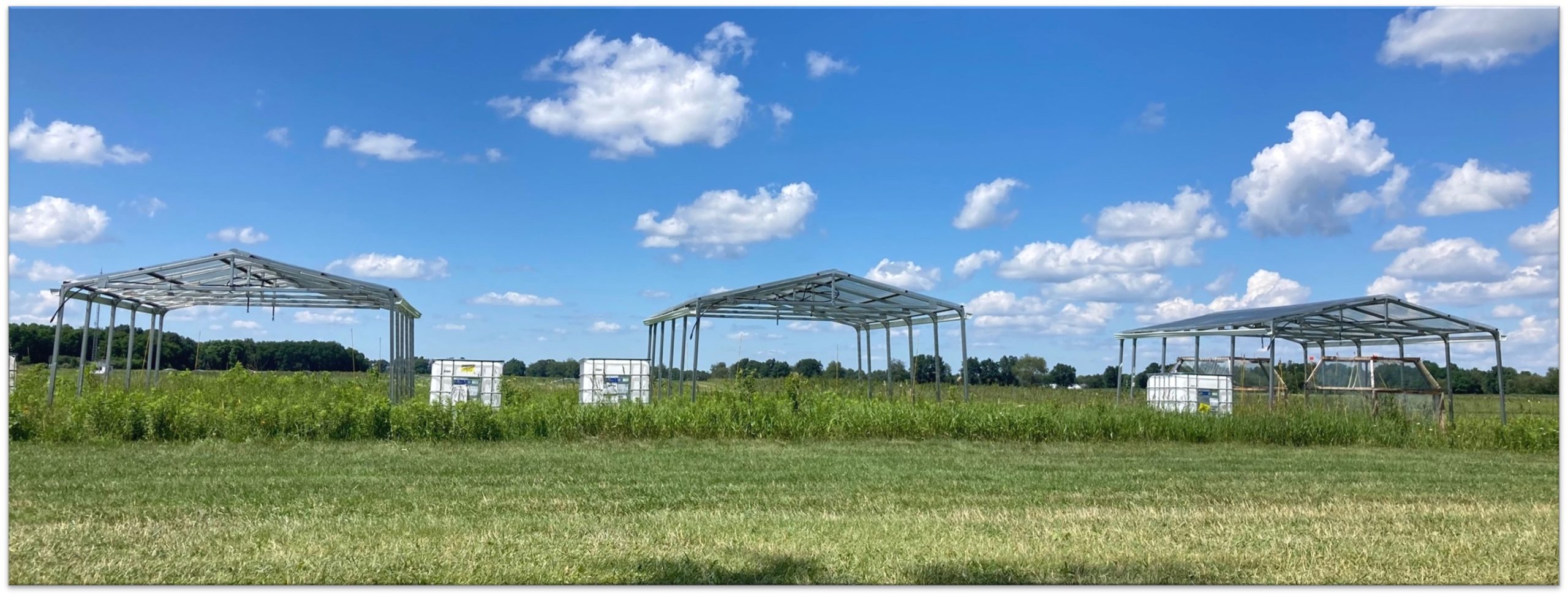
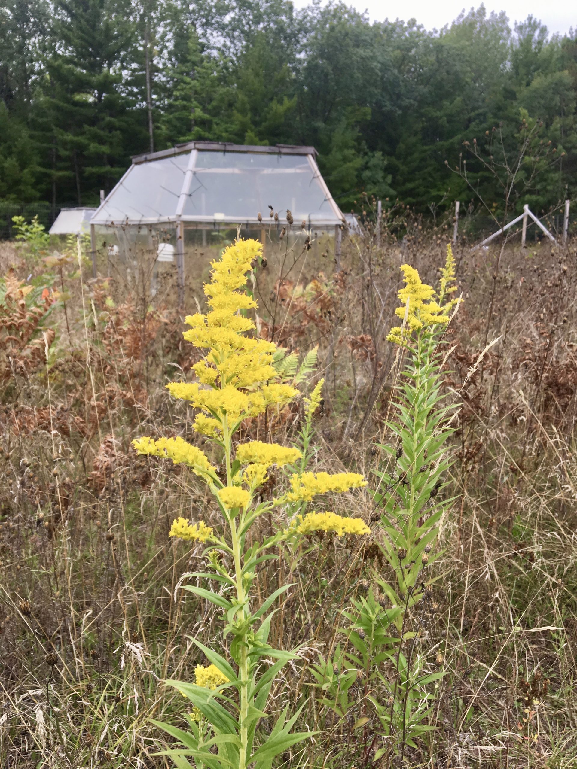
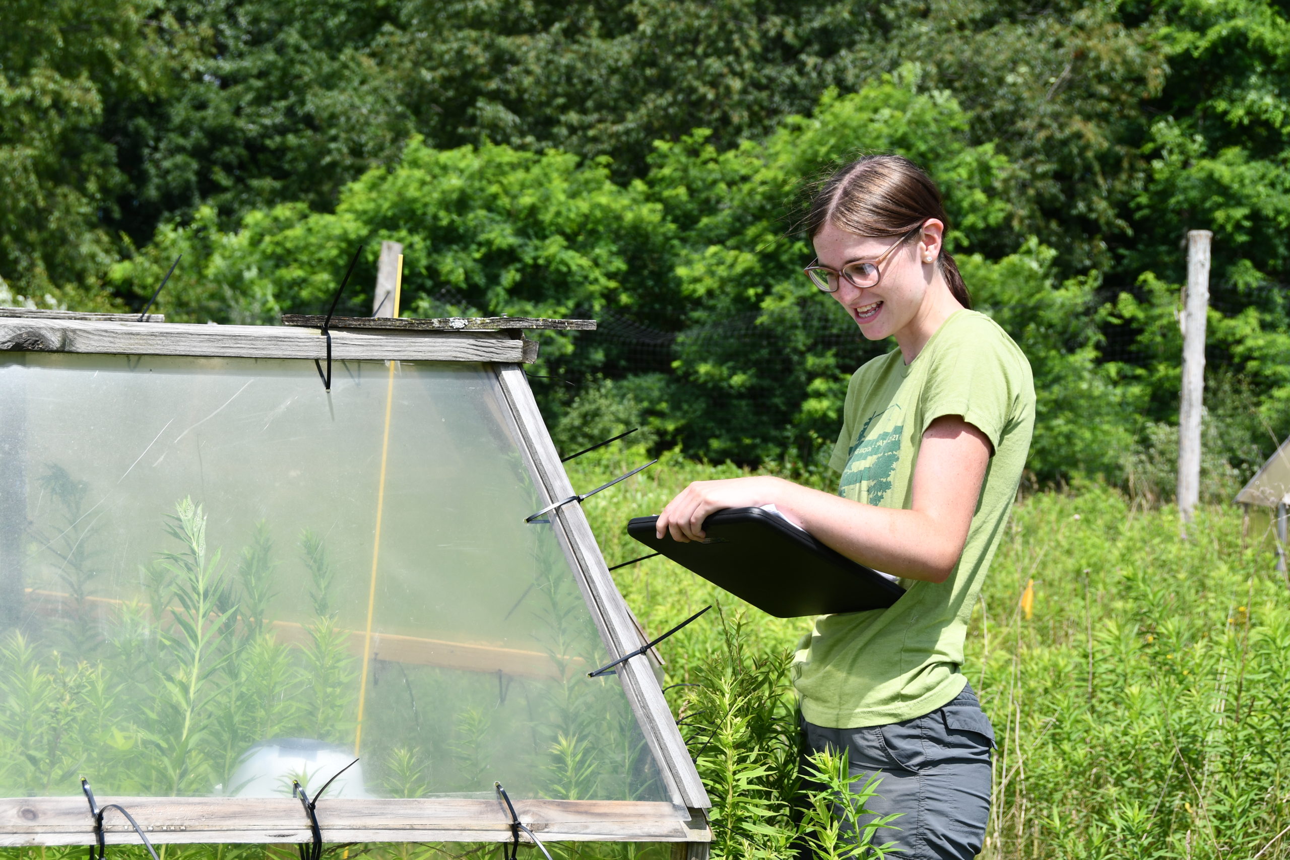
At the Kellogg Biological Station in southwest Michigan, a group of researchers wanted to know how climate warming will affect plant communities. To find out, they created what they call “mini time machines” using open-top chambers. These chambers are clear, hexagonal-shaped structures that trap heat and make the air inside warmer – just like a greenhouse. The chambers still allow for natural levels of precipitation, air flow, and insects to enter through their open tops. By comparing plant communities grown in these warmed conditionswith chambers, to ambient conditions without the chambers, scientists can see how rising temperatures might impact the plants in the future. Understanding these changes can help us prepare for a future where the climate is different from what we know today.
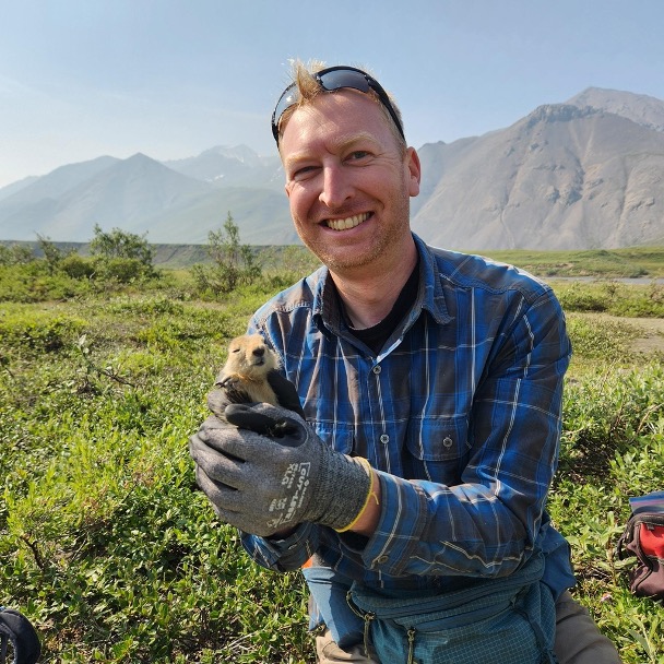
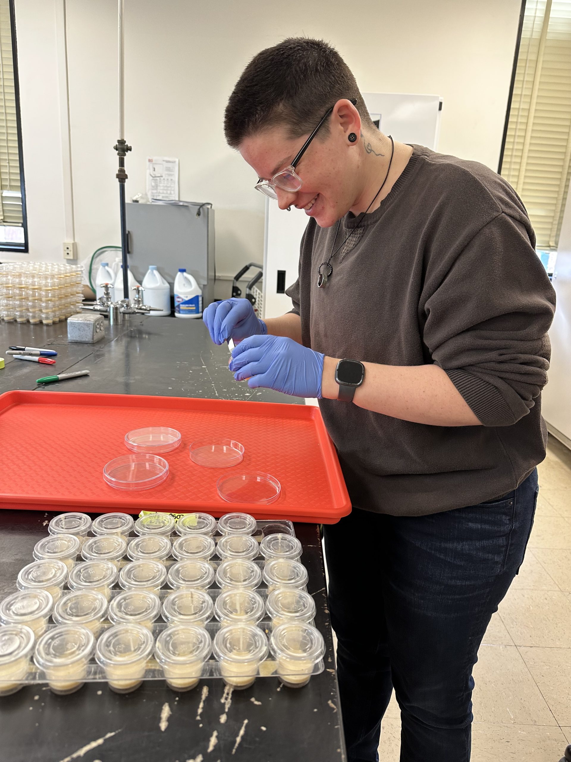
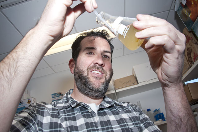
The scientists working in the open-top chambers were at multiple stages in their careers. Moriah is a graduate student who became fascinated with plants when she first learned how to identify different species. Instead of looking at plants as all one patch of green, she could then notice all the diversity and the different roles they play in an ecosystem. Mark is a lab technician working with Moriah. He is interested in how plants will respond to warmer climates because it gives a glimpse of the world his grandchildren will see.
When Moriah and Mark started, they were joined by a few other scientists: Kara, another graduate student, and Emily, an undergraduate student. The open-top chambers had already been out in the field for five years. The field was growing with a diverse mix of plants common in the area. Together, they observed that plants growing in the warmed conditions inside the chambers seemed to be taller than those growing in the ambient conditions outside the chambers.
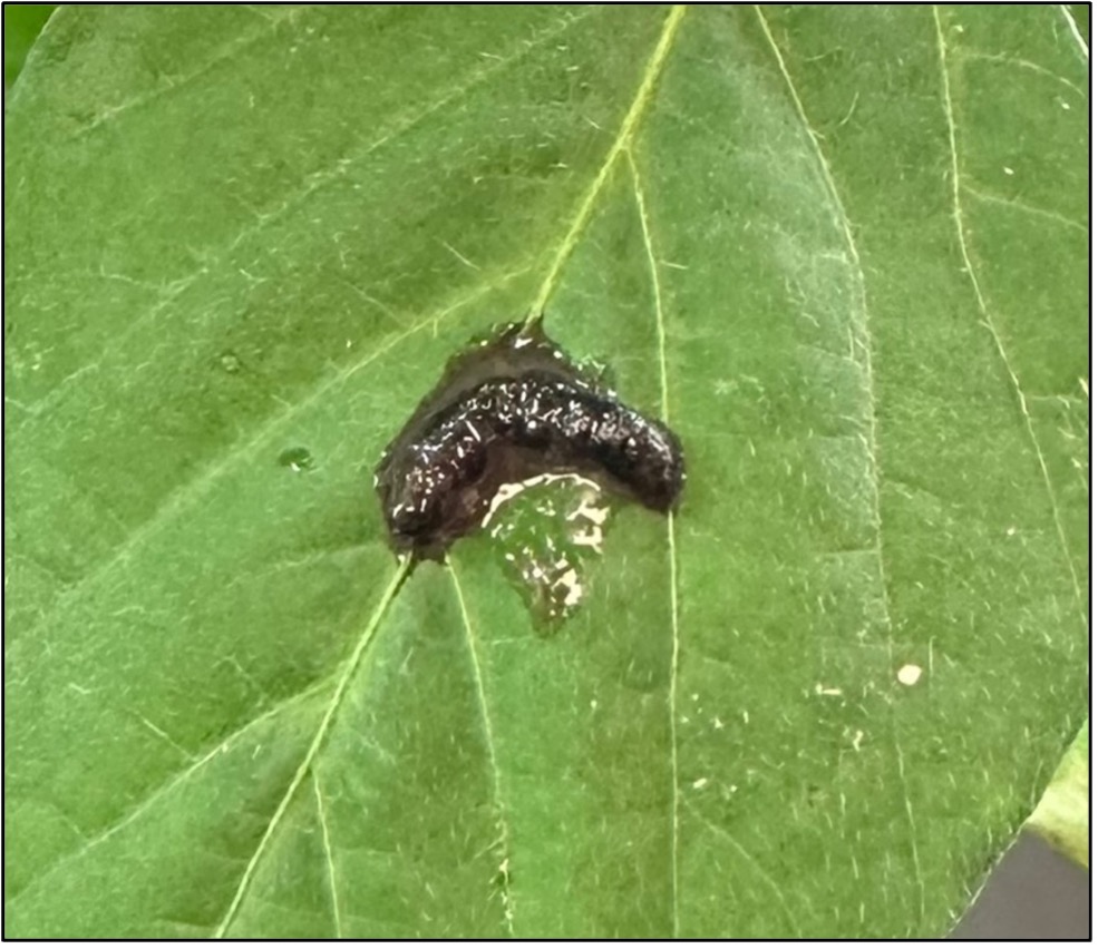
To collect some data to back up their observation, the team began with one species, tall goldenrod. This is a wildflower species with a bright yellow flower, and it is one of the most common species at this location. They wanted to see how goldenrod growth differed in warmed and ambient conditions. When temperatures rise, some plants grow faster and taller to compete for sunlight, but this takes a lot of energy. That means plants have less energy for survival, making seeds, or defending against herbivores, like insects. The researchers predicted that goldenrod inside the chambers would be taller, but would also have fewer stems and plants because they were putting their energy into growing tall instead of making more plants.
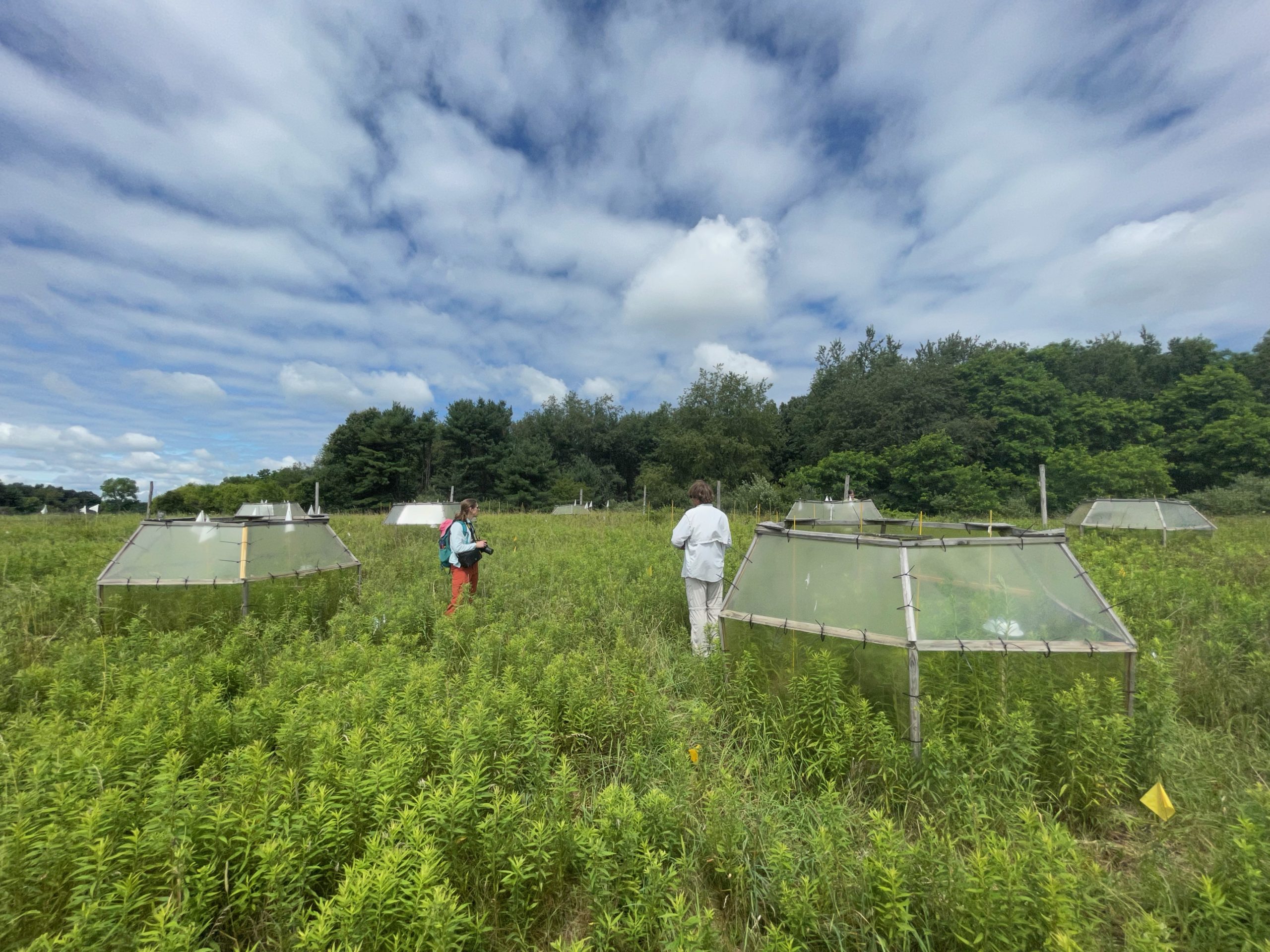
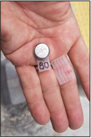
To test their ideas, the team measured goldenrod height with meter sticks and counted the number of goldenrod stems in each plot, called abundance. Their experiment had 30 plots. Half of the plots had open-top chambers, and half did not. That gave them 15 replicates of each treatment. Each plot is 1 meter x 1 meter.
Featured Scientists: Mark Hammond (he/him), Moriah Young (she/hers), Kara Dobson (she/hers), and Emily Parker (she/hers) from the Kellogg Biological Station Long Term Ecological Research Program
Flesch–Kincaid Reading Grade Level = 9.3
Additional Resources:
- The group of researchers featured in this activity work together at the Kellogg Biological Station, part of Michigan State University. Their lab is called the Spatial and Community Ecology Lab (SpaCE Lab). To learn more about their lab and work, students can visit their website or check out the Scientist Profiles associated with this activity.
- Trevor Grabill produced a woodblock printed piece featuring the open-topped chamber experiment, titled What if it’s beautiful?. Along with the piece, they also produced a Zine that includes testimonials by the artist and scientists.