The activities are as follows:
Gena and Ali are sisters who grew up in Bayfield, Wisconsin on the south shore of Lake Superior. When they were young, they spent many summer days sailing in the Apostle Islands National Lakeshore with their parents and friends. As they relaxed on the beach, they would watch how the lake changed. Even over a short period of time, they would see the landscape change. In just a few hours, a rock that was visible above the water’s surface when they arrived would slowly become submerged, only to reappear several hours later.
In high school, Gena and Ali set out to learn about the geophysical forces acting on Lake Superior. They wanted to investigate why they would sometimes see such dramatic fluctuations in water levels. They also wanted to know why water from rivers and streams would sometimes flow out into the lake, while other times it would flow back into the tributaries.
They learned that large lakes exhibit a phenomenon called a seiche (pronounced saysh). Like tides, a seiche is a periodic rising and falling of water levels. However, tides and seiches are caused by two different forces. Whereas tides are connected to the sun and moon, seiches are caused by changes in atmospheric pressure and strong winds.
Many atmospheric events can exert force on the water, including storms that come and go, heavy rain, cold fronts blowing through, or the calming of strong winds. You can think of Lake Superior as a giant bathtub, and the seiche is the water sloshing back and forth as it is pushed by a force and then released.
Gena and Ali realized that the seiche probably explained the water level changes they saw on Lake Superior. They became curious to learn more about the lake’s seiche pattern. An atmospheric event can cause the water to slosh from one side of the lake to the other several times. They predicted the seiche would look like a wave pattern as the water comes and goes.
To test their ideas, they decided to investigate how often the water switched directions and how much the water level changed because of the seiche. In other words, they wanted to measure the amplitude and period of the seiche. The amplitude is the height of a wave from its midpoint, or equilibrium. The amplitude can be calculated as half of the water level change from its highest and lowest point in a cycle. The length of time it takes to complete one full back-and-forth cycle is called the period. You can track the period of the seiche by how much time has passed from one peak to the next peak.
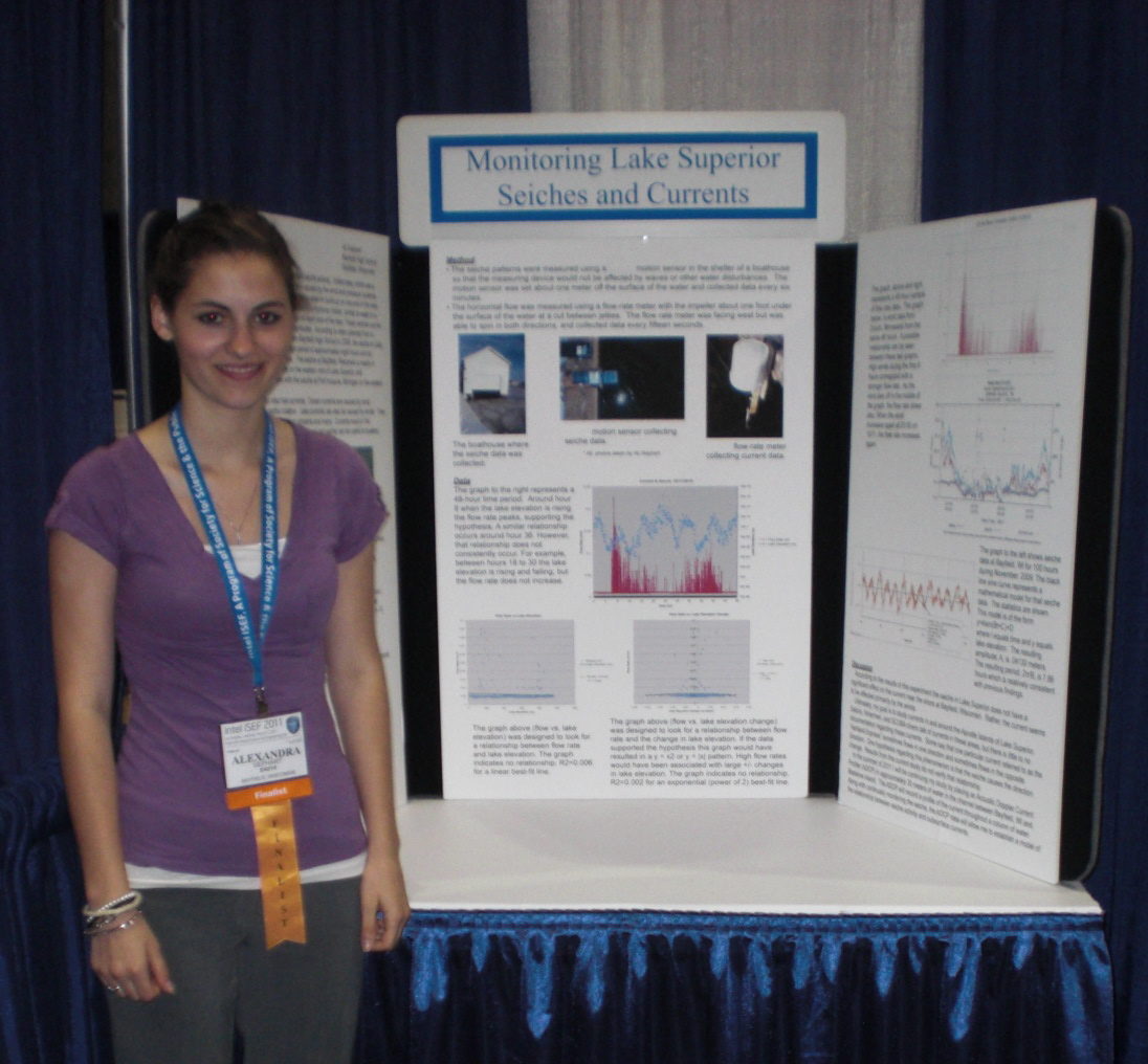
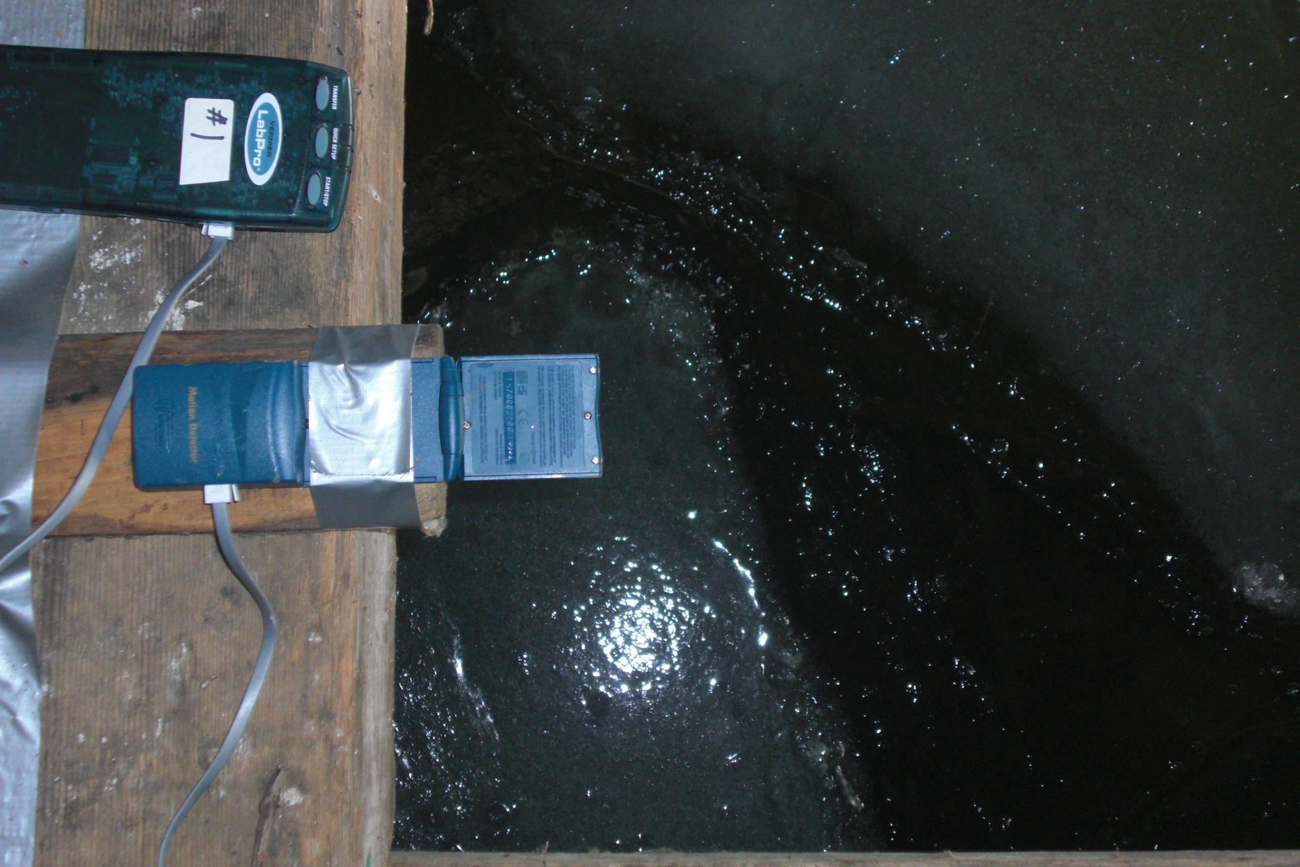
Over their summer break, Gena and Ali started to plan how they could document changes in water levels in their hometown. With permission, Gena and Ali placed a sensor inside a boathouse that was protected from wave action. The sensor measured the distance to the nearest object and was set to collect a data point every six minutes. Gena and Ali placed the sensor so that it faced the surface of the water. That way, it would document changes in the water level throughout time.
Featured scientists: Gena (she/her) and Ali Gephart (she/her), Bayfield High School.
Written by: Richard Erickson, Bayfield High School, and Hannah Erickson, Boston Public Schools.
Flesch–Kincaid Reading Grade Level = 8.8
Additional teacher resources related to this Data Nugget include:
- Here is a link to learn more about the physics of waves.
- Visit this NOAA website to learn more about seiche behavior and characteristics.