The activities are as follows:
- Teacher Guide
- Student activity, Graph Type A, Level 4
- Student activity, Graph Type B, Level 4
- Student activity, Graph Type C, Level 4
- PowerPoint of images
- Grading Rubric
The birds at a beach are very different from those in the forest. This is because each bird species has their own set of needs that allows them to thrive where they live. Habitats must have the right collection of food to eat, places to shelter and raise young, safety from predators, and the right environmental conditions like temperature and moisture.
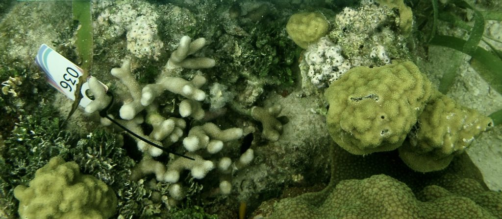
The vast coniferous forests of the Pacific Northwest provide rich and diverse habitat types for birds. These forests are also a large source of timber, meaning they are economically valuable for people. Disturbances from logging and natural events result in a forest that has many different habitat types for birds to choose from. In general, areas of forest that have been harvested more recently will have more understory, such as shrubs and short trees. Old-growth forests usually have higher plant diversity and larger trees. They are also more likely to have downed trees or standing dead trees, which are important for some bird species. Other disturbances like wildfire, wind, large snow events, and forest disease also have large impacts on bird habitat.
At the Andrews Forest Long-Term Ecological Research site in the Cascade Mountains of Oregon, scientists have spent decades studying how the plants, animals, land use, and climate are all connected. In the past, Andrews Forest had experiments manipulating timber harvesting and forest re-growth. This land use history has large impacts on the habitats found in an area. Many teams of scientists work in this forest, each with their own area of research. Piece by piece, like assembling a puzzle, they combine their data to try to understand the whole ecosystem.
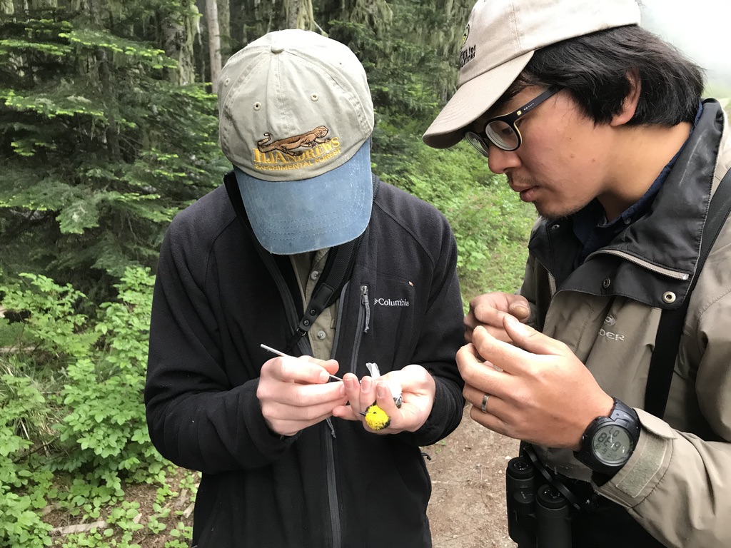
Matt, Sarah, and Hankyu have been collecting long-term data on the number, type, and location of birds in Andrews Forest since 2009. Early each morning, starting in May and continuing until late June, teams of trained scientists hike along transects that go through different forest types. Transects are parallel lines along which data are collected. At specific points along the transect, the team would stop and listen for bird songs and calls for 10 minutes. There are 184 survey locations, and they are visited multiple times each year.
At each sampling point, Matt, Sarah, and Hankyu carefully recorded a count for each bird species that they hear within 100 meters. They then averaged these data for each location along the transect to get an average number for the year. The scientists were also interested in the habitats along the transect, which includes the amount of understory plants and tall trees, two forest characteristics that are very important to birds. They measured the percent cover of understory vegetation, which shows how many bushes and small plants were around. They also measured the size of trees in the area, called basal area.
Using these data, the research team is looking for patterns that will help them identify which habitat conditions are best for different bird species. With a better understanding of where bird species are successful, they can predict how changes in the forest could affect the number and types of birds living in Andrews Forest and nearby.
Wilson’s Warblers and Hermit Warblers are two of the many songbirds that these scientists have recorded at Andrews Forests. Wilson’s Warblers are small songbirds that make their nests in the understory of the forests. Therefore, the team predicted that they would see more of Wilson’s Warblers in forest areas with more understory than in forest areas with less understory. Hermit Warblers, on the other hand, build nests in dense foliage of tall coniferous trees and search for spiders and insects in those coniferous trees. The team predicted that the Hermit Warblers would be observed more often in forest plots where there are larger trees.
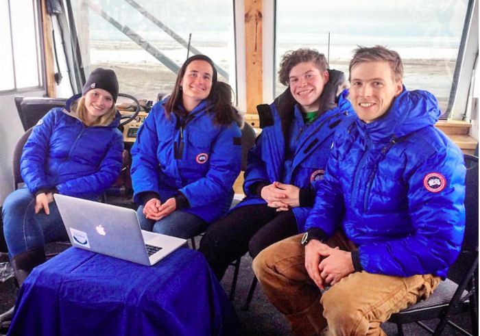
Featured scientists: Hankyu Kim, Matt Betts, and Sarah Frey from Oregon State University. Written with Eric Beck from Realms Middle School and Kari O’Connell from Oregon State University.
Flesch–Kincaid Reading Grade Level = 10.5
Additional teacher resource related to this Data Nugget:
- A slideshow of the images is available for this activity.
- To access more data, and learn more about the H.J. Andrews Long Term Ecological Research site, check out their website.