The activities are as follows:
- Teacher Guide
- Student activity, Graph Type A, Level 2
- Student activity, Graph Type B, Level 2
- Student activity, Graph Type C, Level 2
- Grading Rubric
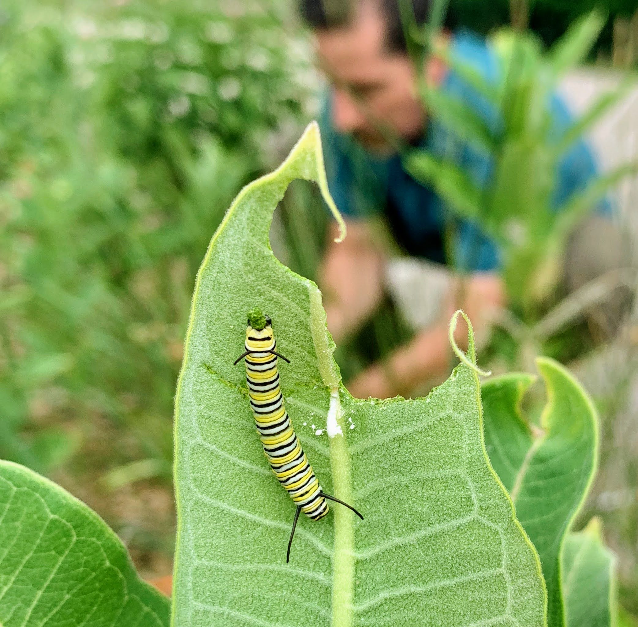
The North American Bison is an important species for the prairie ecosystem. They are a keystone species, which means their presence in the ecosystem affects many other species around them. For example, they roll on the ground, creating wallows. Those wallows can fill up with water and create a mini marsh ecosystem, complete with aquatic plants and animals. They also eat certain kinds of food – especially prairie grasses. What bison don’t eat are wildflowers, so where bison graze there will be more flowers present than in the areas avoided by bison. This affects many insects, especially the pollinators that are attracted to the prairie wildflowers that are abundant in in the bison area.
Not only do bison affect their environment, but they are also affected by it. Because bison eat grass, they often move around because the tastiest meals might be scattered in different areas of the prairie. Also, as bison graze down the grass in one area they will leave it in search of a new place to find food. The amount of food available is largely dependent upon the amount of rain the area has received. The prairie ecosystem is a large complex puzzle with rain and bison being the main factors affecting life there.
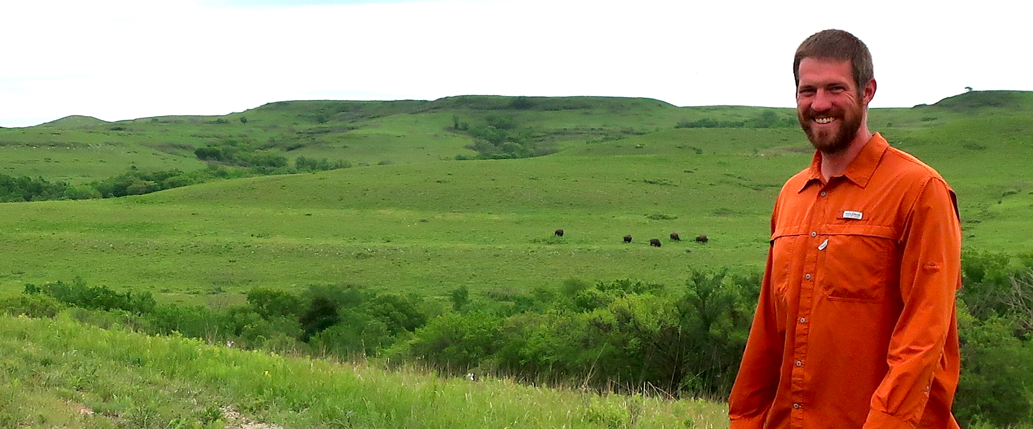
The Konza Prairie Biological Station in central Kansas has a herd of 300 bison. Scientists study how the bison affect the prairie, and how the prairie affects the bison. Jeff started at Konza as a student, and today he is the bison herd manager. As herd manager, if is Jeff’s duty to track the health of the herd, as well as the prairie.
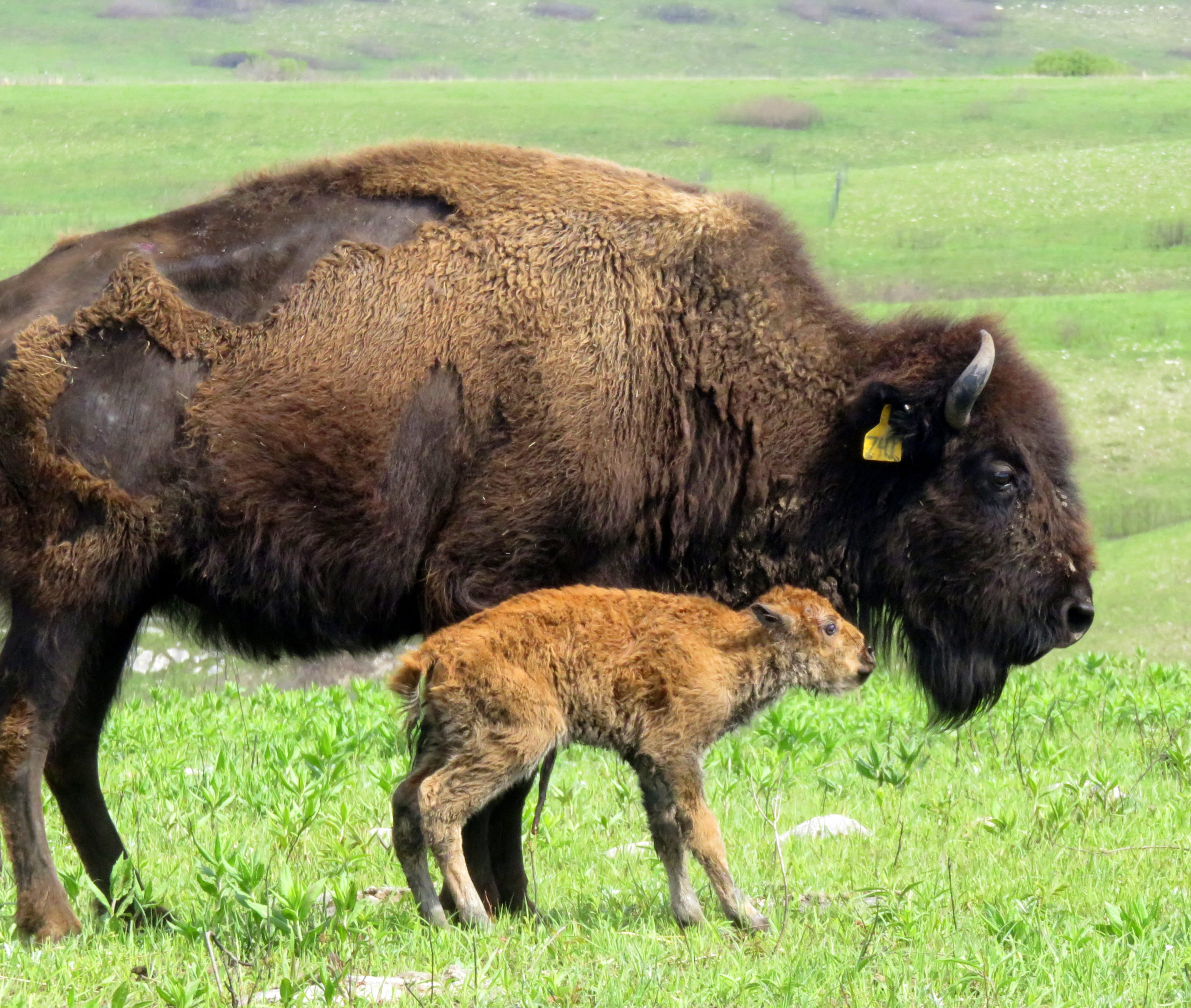
One of the main environmental factors that affect the prairie’s health is rainfall. The more rain that falls, the more plants that grow on the prairie. This also means that in wetter years there is more food for bison to eat. Heavier bison survive winters better, and then may have more energy saved up to have babies in the following spring. Jeff wanted to know if a wet summer would actually lead to healthier bison babies, called calves, the following year.
Jeff and other scientists collect data on the bison herd every year, including the bison calves. Every October, all the bison in the Konza Prairie herd are rounded up and weighed. Since most of the bison calves are born in April or May, they are about 6 months old by the time are weighed. The older and the healthier the calf is, the more it weighs. Very young calves, including those born late in the year, may be small and light, and because of this they may have a difficult time surviving the winter.
Jeff also collects data on how much rain and snow, called precipitation, the prairie receives every year. Precipitation is measured daily at the biological station and then averaged for each year. Precipitation is important because it plays a direct role in how well the plants grow.
Featured scientist: Jeff Taylor from the Konza Prairie Biological Station
Written by: Jill Haukos, Seton Bachle, and Jen Spearie
Flesch–Kincaid Reading Grade Level = 8.7
Additional teacher resources related to this Data Nugget include:
- The full dataset for bison herd data is available online! The purpose of this study is to monitor long-term changes in individual animal weight. The datasets include an annual summary of the bison herd structure, end-of-season weights of individual animals, and maternal parentage of individual bison. The data in this activity came from the bison weight dataset (CBH012).
- For more information on calf weight, check out the LTER Book Series book, The Autumn Calf, by Jill Haukos.