The activities are as follows:
- Teacher Guide
- Student activity, Graph Type A, Level 3
- Student activity, Graph Type B, Level 3
- Student activity, Graph Type C, Level 3
- Grading Rubric
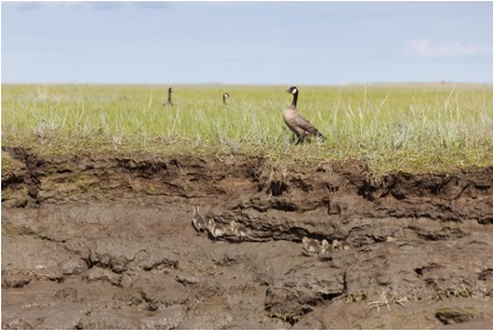
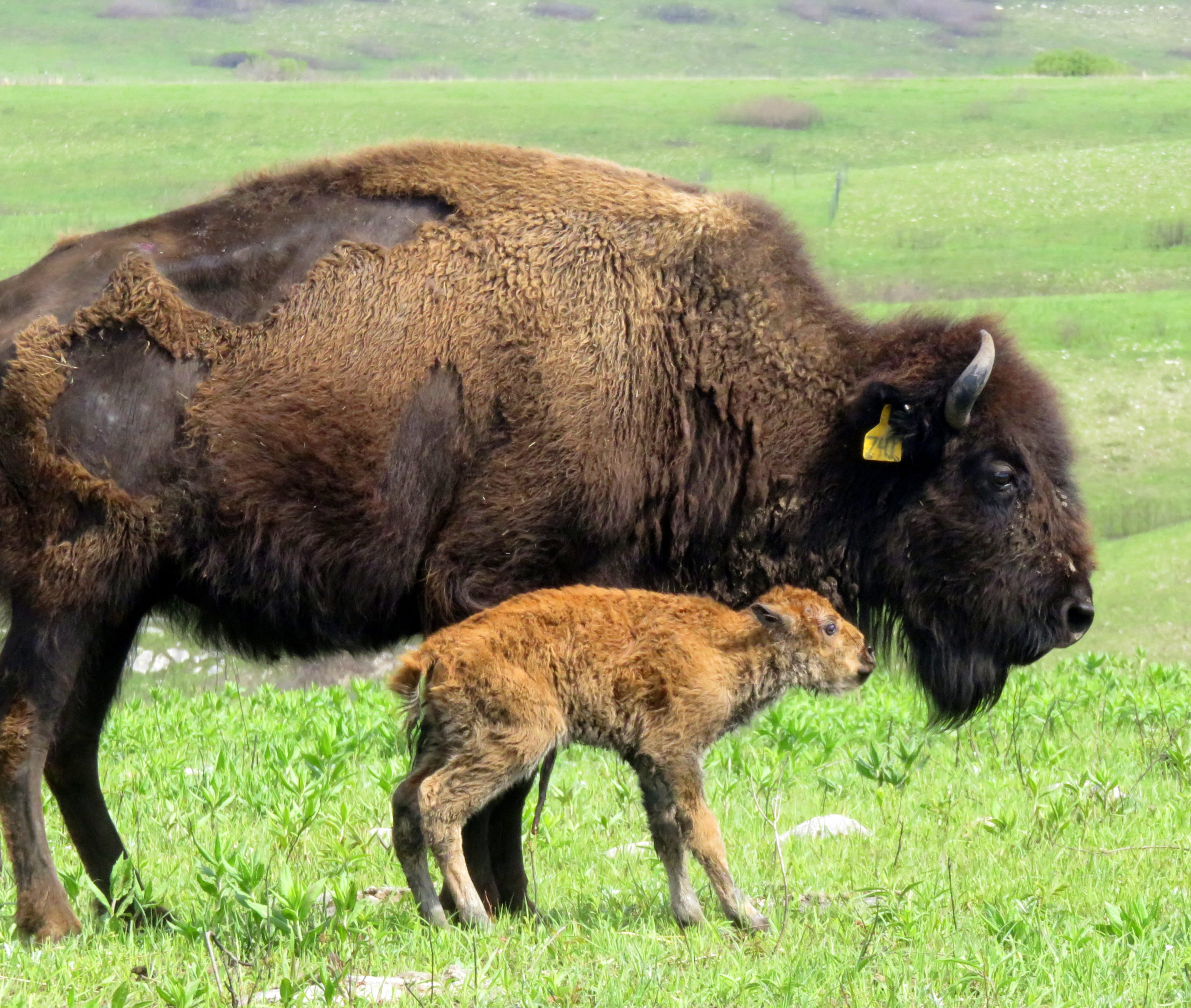
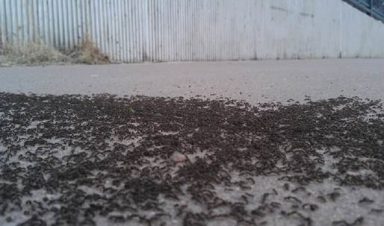
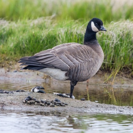
Each spring, millions of birds return to the Yukon-Kuskokwim Delta. This delta is where two of the largest rivers in Alaska empty into the Bering Sea. It is also one of the world’s most significant habitats for geese to breed and raise their young.
With all these geese coming together in one area, they create quite a mess – they drop tons of poop onto the soil. So much poop in fact, that scientists wonder whether poop from this area in Alaska could have a global impact! Climate change is a worldwide environmental issue that is caused by too many greenhouse gasses being released into our atmosphere. Typically, we think of humans as the cause of this greenhouse gas release, but other animals can contribute as well.
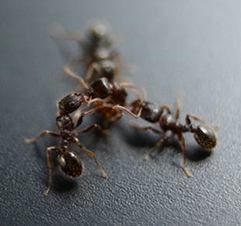
When poop falls onto the soil it is decomposed by bacteria. Bacteria release methane (CH4), a potent greenhouse gas. The more geese there are, the more poop they will produce and the more food there will be for soil bacteria. By increasing the amount of greenhouse gasses that are released by soil bacteria, geese might actually indirectly contribute to global climate change.
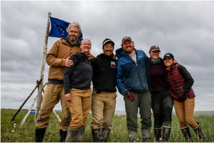
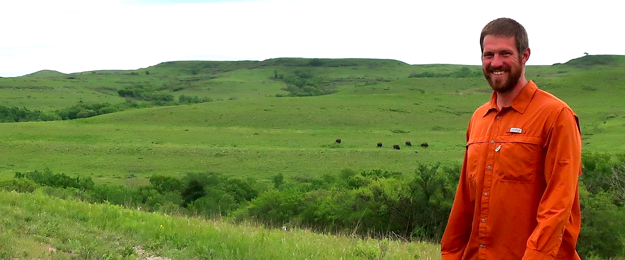
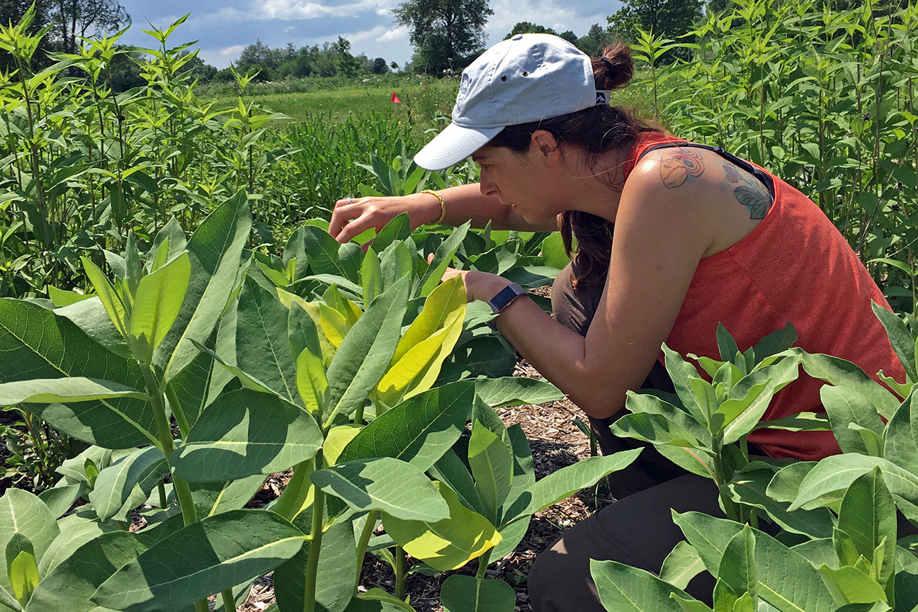
Trisha is an ecosystem ecologist who scoops goose poop for research projects. Her research is looking into whether animals, other than humans, can change the carbon cycle. Trisha teamed up with Bonnie, a fellow ecosystem ecologist. Bonnie studies how matter moves between the living parts of the environment, such as plants and animals, and the nonliving parts. She is especially interested in how bacteria in the soil play a role in the carbon cycle.
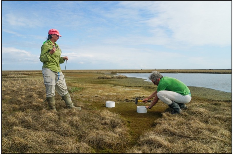
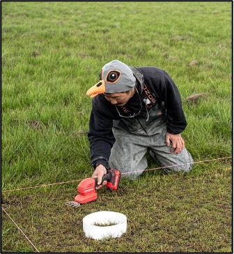
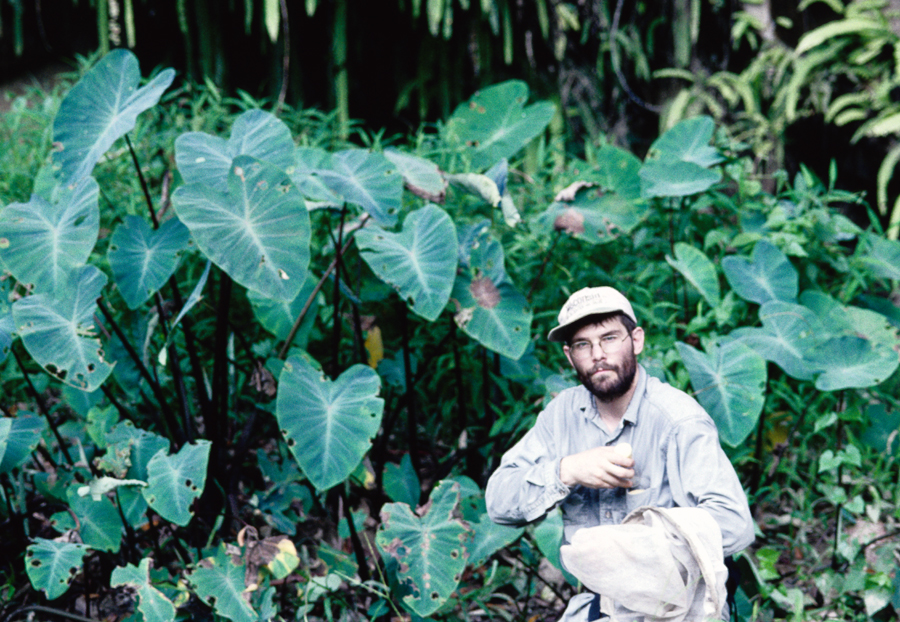
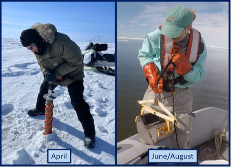
Together, the team designed a three-year project to figure out the effects of goose poop on the carbon cycle. Each summer, a large team of researchers spend 90 days camping on remote sites near the Yukon-Kuskokwim Delta. The team scooped up poop from nearby goose habitats to use in their experiments. They set up six control plots where they added no poop and six treatment plots where they added poop. From these twelve plots, the team measured methane emissions from the soil. Methane was measured as methane flux in micromoles, or µM. These data helped them determine how ecosystems respond to geese by measuring whether goose poop affects methane production by soil bacteria.
Featured scientists: Trisha Atwood of Utah State University and Bonnie Waring of Imperial College. Written by Andrea Pokrzywinski.
Flesch–Kincaid Reading Grade Level = 8.7
Additional teacher resources related to this Data Nugget include:
- This scientist team has done an extensive amount of work that is related to ideas in this Data Nuggets activity. They have many videos, photos, and blog posts up on their shared website for this project, “Geese and the carbon cycle”
- There is one paper associated with the data in this activity:
- Fienup-Riordan, Ann. “Yaqulget Qaillun Pilartat (What the Birds Do): Yup’ik Eskimo Understanding of Geese and Those Who Study Them.” Arctic, vol. 52, no. 1, 1999, pp. 1–22. JSTOR.
- You can also have students complete another Data Nugget in this same system that looks at the impacts of goose poop on the carbon cycle, called “Sink or source? How grazing geese impact the carbon cycle”.
- A video interview featuring scientist Bonnie Waring, talking students through climate change and the role of greenhouse gasses
- Video Interview with scientist Trisha Atwood
- Birds, Plants, and Climate Transform the YK Delta