The activities are as follows:
- Teacher Guide
- Student activity, Graph Type A, Level 4
- Student activity, Graph Type B, Level 4
- Student activity, Graph Type C, Level 4
- Grading Rubric
Most of our energy in the United States comes from fossil fuels like natural gas, coal, and oil. These energy sources are efficient, but they release greenhouse gases into the atmosphere when burned. They are also non-renewable, meaning there is a limited supply. Renewable energy options collect energy from sources that are naturally replenished, such as sunshine, wind, and even ocean waves. By using renewable energy sources, we can fuel our lives without depleting fossil fuel supplies.
Windmills have been used by humans to capture energy from the wind long before electricity was discovered. Historically, they were used to pump water and grind grains to make flour. Today, they are used to generate electricity that can be used in your home. Most of these modern windmills (also known as turbines) are located on land, but researchers and engineers are exploring a new type of site – the ocean.
Offshore wind energy sites in the U.S. are usually at least 20 miles from land. Winds that blow over the ocean are much more consistent than on land, making offshore energy more reliable. In addition, land that can be used for windmills is limited, especially in areas where there are already a lot of people. Offshore wind energy could be a solution where there are a lot of people living along the coast.
Careful planning goes into these large-scale projects. Before any construction begins, scientists want to make sure the benefits outweigh the costs. One topic of concern is marine mammals. Many marine mammals, like whales, are federally protected, and some are endangered species. Scientists are worried that the construction of offshore windmills could impact the whales that live or migrate through the designated wind energy areas.
Whales use sound transmitted through the water to survive. Just like many animals on land, they use sound to communicate, navigate, find food, and avoid predators or other threats. Noise from construction activities could cause whales to avoid the area. They may need to find a new area to find food, rest, or find mates. Whales typically migrate, so loud noises could also interfere with their migration route.
Shannon is an acoustic ecologist, meaning she uses sound and how it is transmitted to learn more about organisms and their environment. She works with Desray, who is a research biologist specializing in marine mammals. Together, they are leading a large project to collect sound data to assess the risks of a proposed offshore wind energy site off the coast of central California. One specific goal they have is to see whether it is possible to identify the best time of year to build the wind energy platforms with the least disturbance to marine mammals. To do this, they had to learn more about when whales are using and traveling through the area of the proposed site.
Acoustic ecology is a way to learn more about whales and their behavior through sound, which is important because visual detections are limited and take a lot of time out at sea. Instead, scientists can analyze acoustic data to detect which species are present. Each species makes different sounds with unique patterns, and by listening, we can identify which species are in the area.
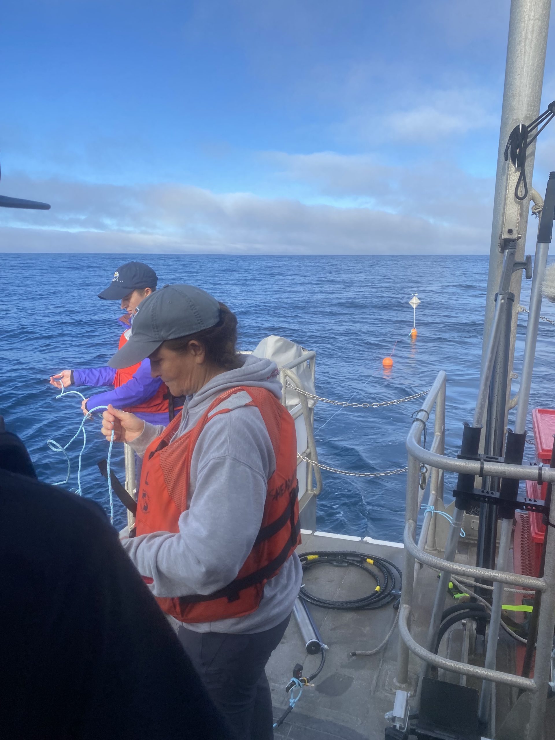
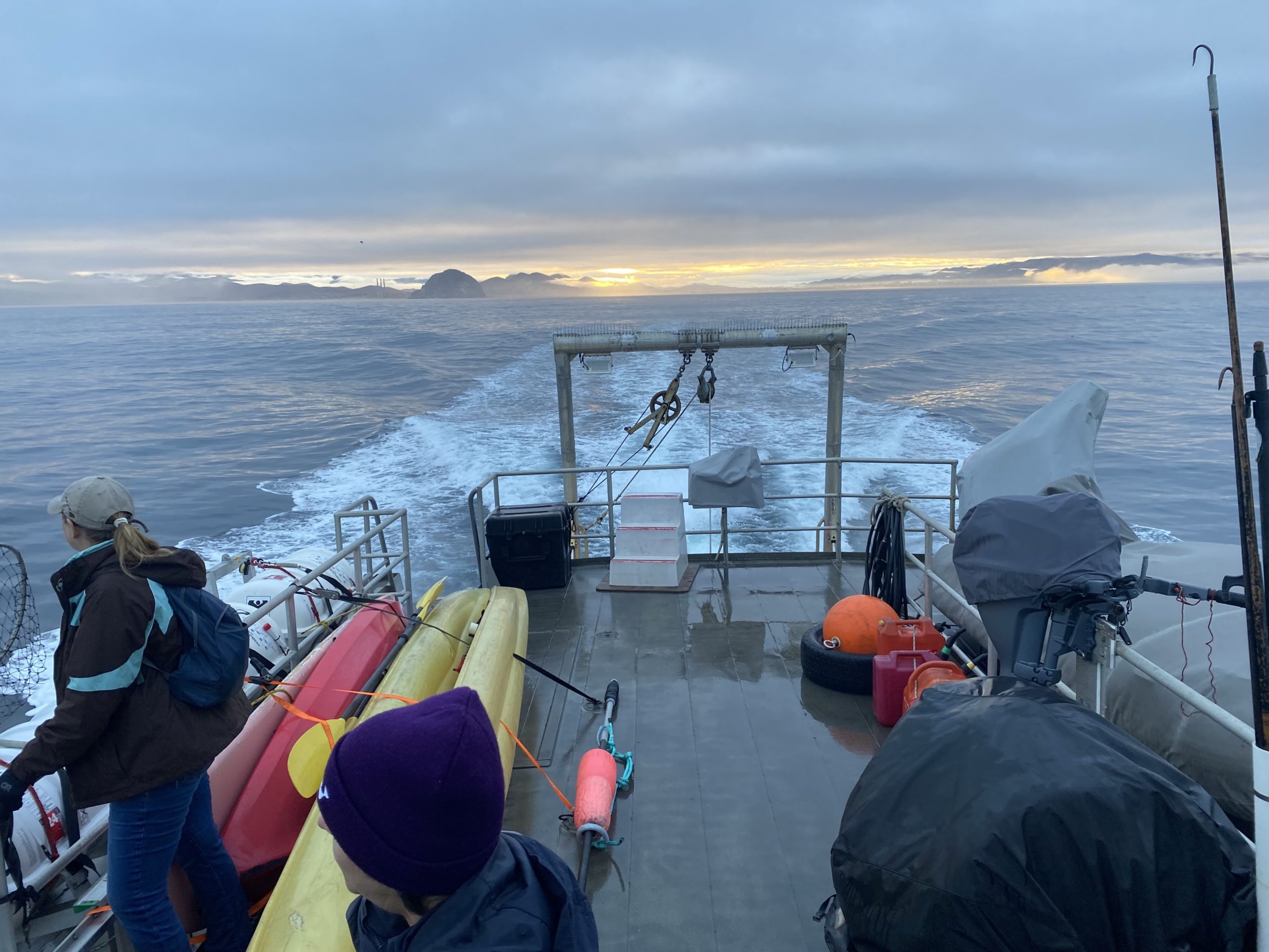
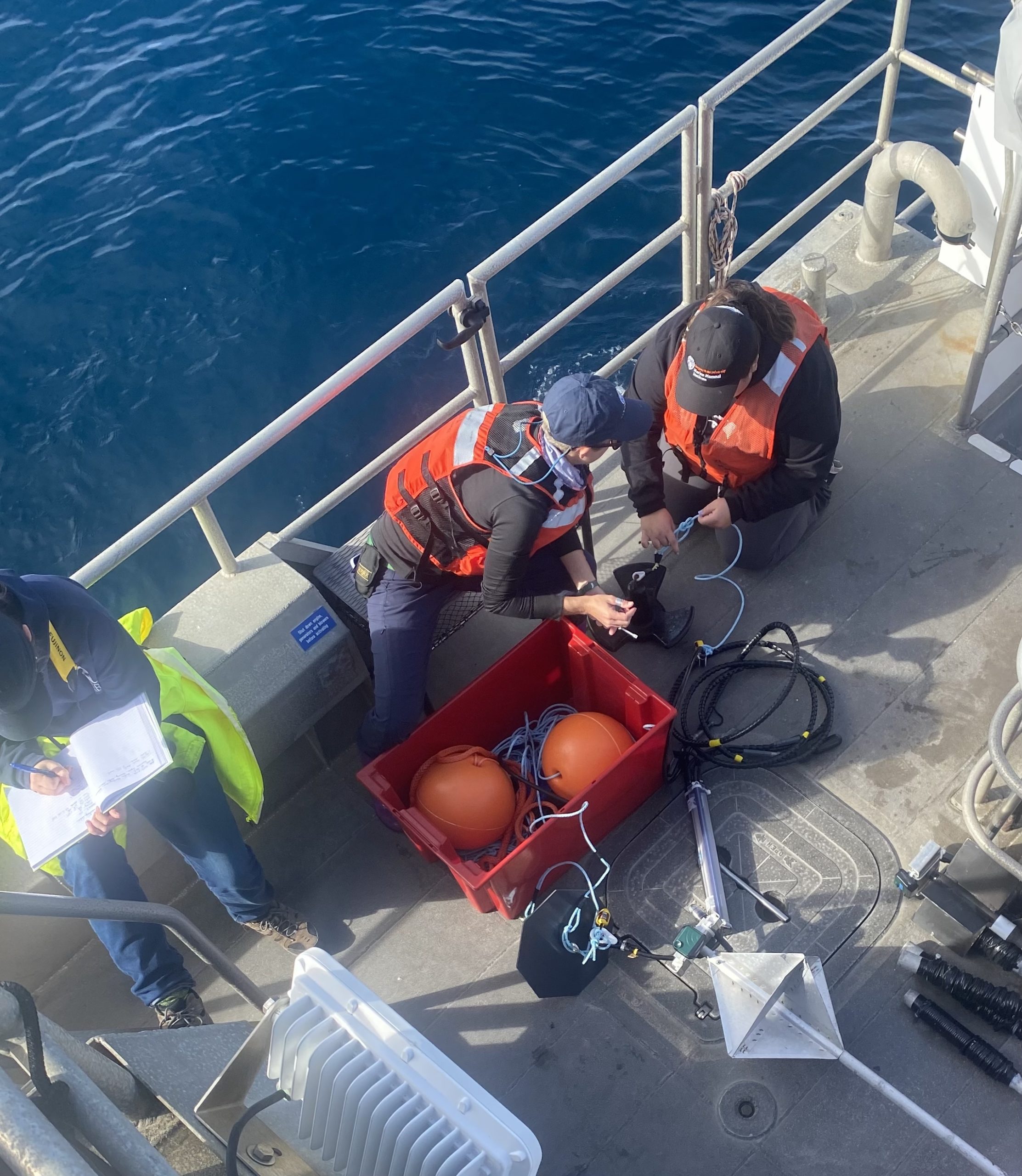
Shannon and a large team of supporting scientists worked together to design floating acoustic recorders. They partnered with Desray to deploy them in the proposed offshore wind energy area. Once the recorders are launched, the team uses satellite location to follow the movement of the recorders from shore. They let the recorders drift in the open ocean for several days before they board a large research boat and pick them up again. While the recorders are drifting, they are continuously recording the ocean sounds below. These drifting recorders cover a larger spatial area, for a longer time, than other types of passive acoustic monitoring methods. The team launched the acoustic recorders in different seasons to learn which whale species are using the proposed site throughout the year and to assess what time of year would have the lowest whale presence near the construction site.
Featured scientists: Shannon Rankin from the NOAA Southwest Acoustic Ecology Lab and Desray Reeb from the Bureau of Ocean Energy Management
Flesch–Kincaid Reading Grade Level 9.4
Additional teacher resources related to this Data Nugget:
- The NOAA team members on this project have put together a blog series, called “Sound Bytes,” to share the stories and impacts of the ADRIFT research highlighted in this activity. This blog series features many perspectives showcasing how underwater sound, in the form of acoustic data, can be used to learn more about marine mammals.
- Students can learn more about how acoustic data is analyzed and what it looks like visually by checking out the Ocean Voices project on Zooniverse. Here they can participate in a guided introduction to humpback whale and ship sounds from drifting acoustic recorders and help scientists classify sounds on the recordings.
- These data were collected as part of the ADRIFT project, led by the Southwest Acoustic Ecology Lab run by the National Oceanic and Atmospheric Administration and the Bureau of Ocean Energy Management.
- NOAA has a wide variety of lesson plans that you could use to supplement this activity. Here is a set of activities for elementary, middle, and high school on bioacoustics.
- Lesson on bioacoustics by Seagrant and Woods Hole Oceanographic Institute.
- For more lessons and activities about wind energy, check out the K-12 teaching materials by the Office of Energy and Renewable Energy.
- A collection of videos that show the spectrograms and audio recordings for various marine mammals that you could share with students.
- There is an extensive PowerPoint that has additional information about the ADRIFT acoustics project and other research being done.
This study was funded in part by the U.S. Department of the Interior, Bureau of Ocean Energy Management through Interagency Agreement M20PG00013 with the U.S. Department of Commerce, National Oceanic and Atmospheric Administration, National Marine Fisheries Service (NMFS), Southwest Fisheries Science Center (SWFSC).