Cracks in the Arctic tundra landscape

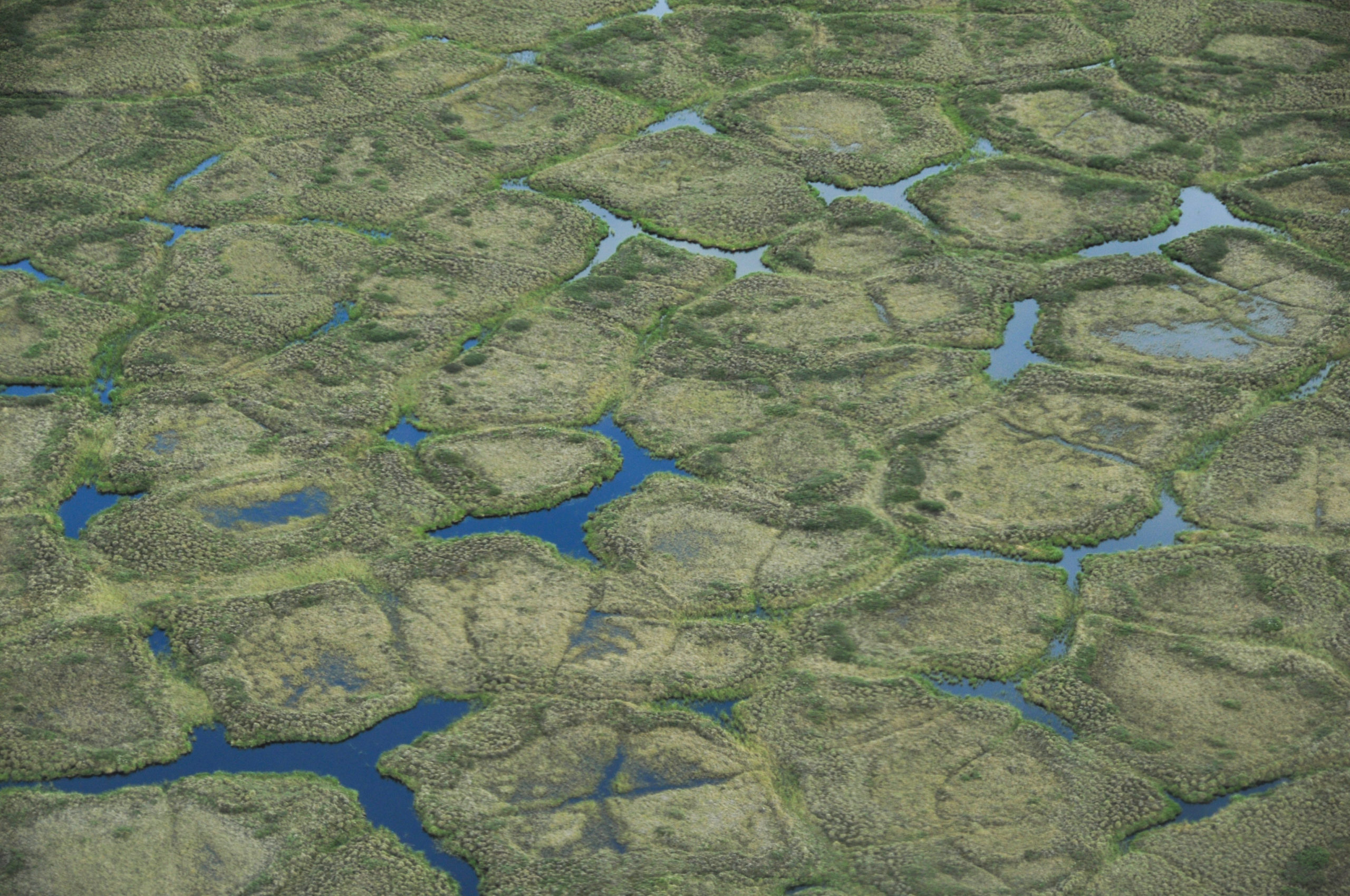
An aerial photograph of an ice-wedge polygon landscape. Photo Credit: U.S. Geological Survey – Christian Zimmerman.

There is a strange phenomenon found in many Arctic regions. There, the natural landscape often has large repeating patterns called ice-wedge polygons. Understanding why they exist and how they form has been a puzzle for many years.

Today, scientists believe ice-wedge polygons form because of the extreme temperature swings in the arctic climate. During the cold winter, the soil contracts and cracks. In summer, water fills these cracks. When temperatures drop again in the fall, the water freezes and expands. Over many years, repeated cycles of cracking and freezing create large wedges of ice underground. These ice wedges connect to form polygon-shaped patterns across the landscape.

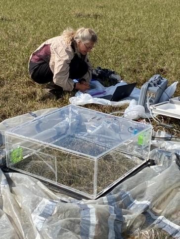
Anja using an infrared gas analyzer in the field.

As they continue to grow, the wedges create microhabitats, or small areas that are close to each other, but differ in physical conditions. The polygons have wet centers, slightly raised and drier rims, and water-filled troughs around the edges. The microhabitats affect water movement, nutrient distribution, carbon cycling, biodiversity, and habitat for animals. The polygon microhabitats are also important carbon sinks – meaning the plants living there take in and store more carbon than they release.

Anja is a scientist working in the Arctic. She first became interested in the connections between plants, soil, and ice when she hiked across the Arctic tundra in northern Alaska for her graduate school research. She got her rubber boots stuck in the deep troughs of the melting ice covering the land. While getting unstuck, she observed the ice-wedge polygons and became curious about the plants that live in each area of the polygons. She was curious whether each microhabitat influences how carbon moves between the land and the atmosphere.

Anja wanted to investigate how much carbon is absorbed by different microhabitats within the polygons. Plants take up carbon dioxide (CO2) from the atmosphere during photosynthesis and use it to build new plant material. She observed that different plant communities grew in different areas of the polygons. The polygon rims have more shrubs and are drier. The troughs have more sedges, which are similar to grasses, and seem to have the wettest conditions. The centers have sedges and moss communities and are wet, but not as wet as the troughs. She thought that the wet plant communities found in the polygon centers would absorb the most carbon because their soil moisture conditions are most favorable for photosynthesis. The conditions in the dry rims and flooded troughs could be more stressful for plants to grow in.

Anja hiked across the Alaskan Arctic tundra at the height of summer again. She marked the location of several well-developed ice-wedge polygons and identified the center, rim, and trough microhabitats within each polygon. She set up three plots in each type of microhabitat as replicates. 

To measure carbon flux, Anja used a clear chamber connected to an infrared gas analyzer. This instrument measured net ecosystem productivity (NEP), which shows the balance of carbon taken up through photosynthesis and released through respiration. Anja used this instrument to measure the amount of CO2 moving into or out of the atmosphere each second over a square meter within each plot.

Featured scientist: Anja Kade (she/her) from University of Alaska Fairbanks

Flesch–Kincaid Reading Grade Level = 10.1

Flowers chasing spring

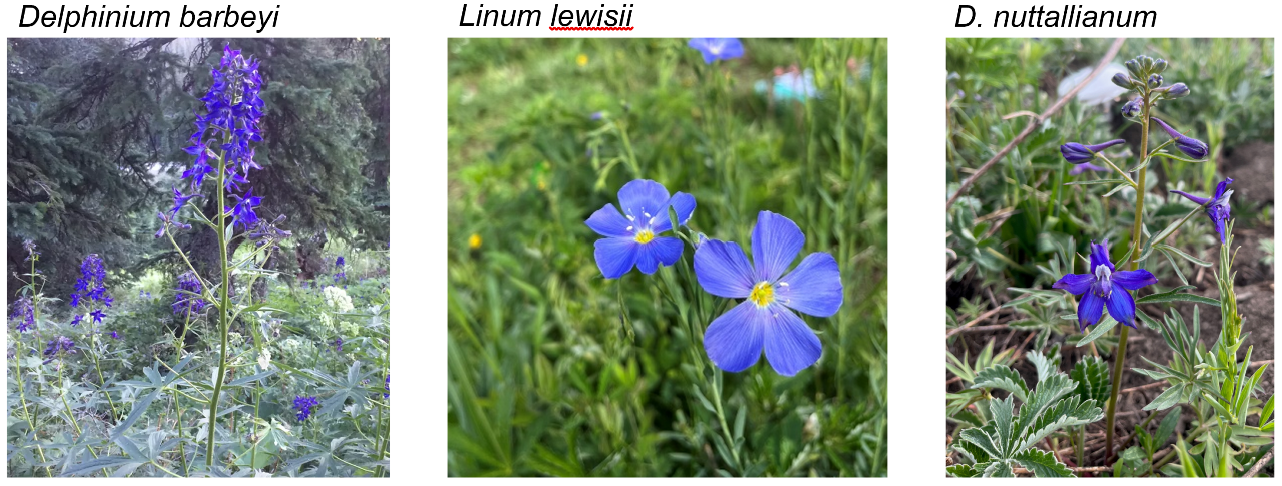
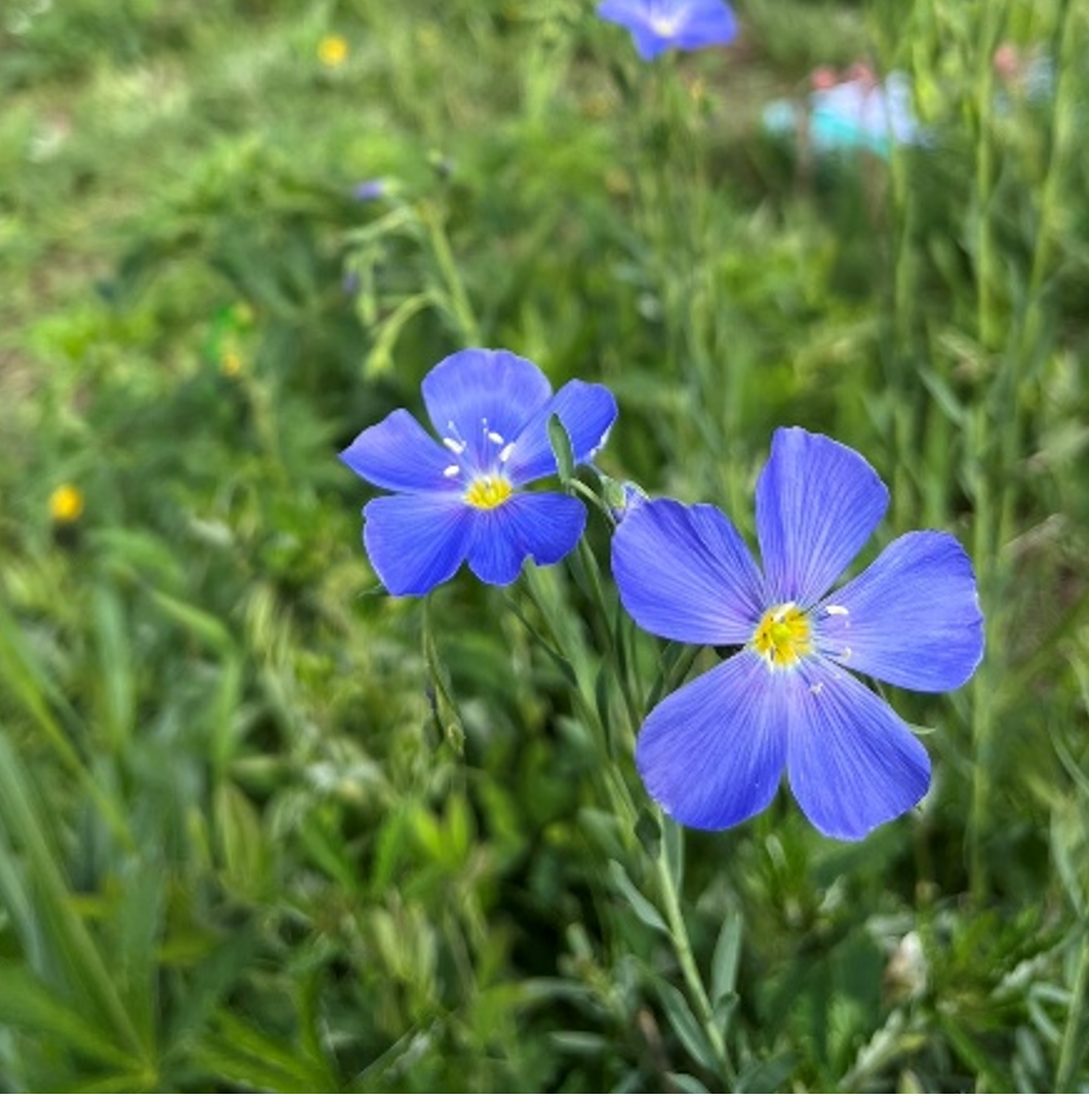
Linum lewisii flower

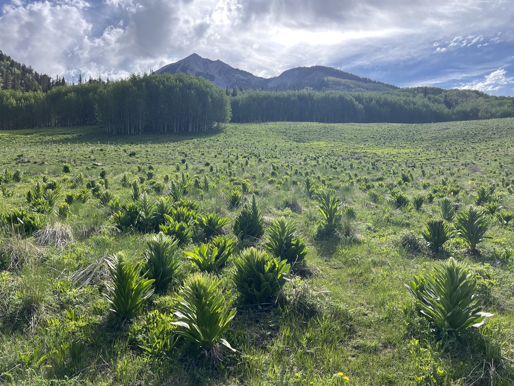
How does a plant know when to make a flower? Their phenology, or seasonal timing of growth and reproduction, can be driven by many things. When the weather warms in the spring, many plants start to make flowers when temperatures are just right. Other plants follow the number of hours with sunlight. In one very particular system, plants might actually be following the timing of snow.

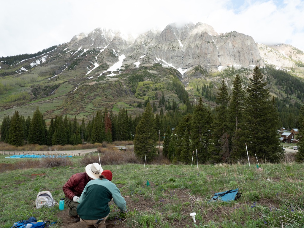
High up in the Rocky Mountains, scientists are studying plants at elevations where snow covers the ground for six months of the year. In the spring, when the ground is still covered in snow. Plants under the snow are unable to sense the temperature of the air or sunlight hours. This means that plants may have to use a different cue, such as the timing of snowmelt, to know when to flower. 

Amy and Dylan are two scientists who love and have spent a lot of time in the Rocky Mountains. While there, they noticed the springs were changing and wanted to document what they were observing. They wondered whether the date of snowmelt was changing over time. If so, were the plants responding by shifting their flower timing?

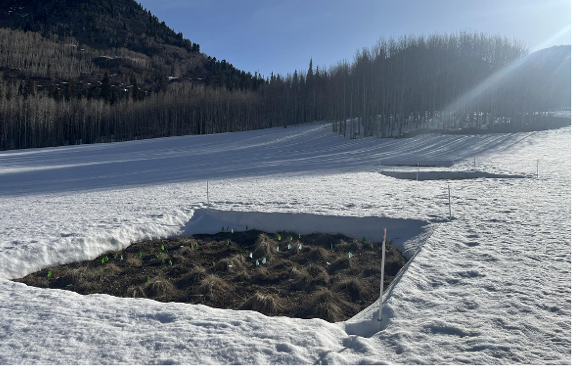
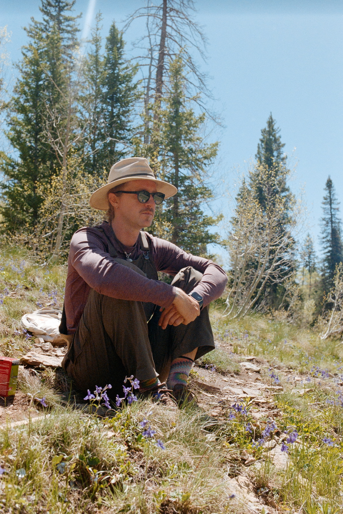
Dylan and a field technician, Mairin Boshoven, observing plants in the Rocky Mountains.

To answer their question, they looked to the work of two additional scientists. The first is David Inouye, a retired plant ecologist from the University of Maryland. David has been observing flowers at the Rocky Mountain Biological Laboratory for the last 50 years. David and his team measured phenology of 163 plant species across 36 plots in the Rocky Mountains. From early spring through summer, they surveyed their plots every two days, recording every plant species flowering in each plot. They measured first flowering date as the day they observed the first flower for each species. His records show, over time plants have been flowering earlier and earlier each year.

Another scientist, billy barr (who doesn’t capitalize his name), has been living and working at the Rocky Mountain Biological Laboratory since the 1970s. Initially for his own curiosity, billy started recording the weather at the Lab. He then built a weather station outside his cabin. His records have become important to many areas of research at the station. 

These records include billy’s observations for the first date that snow was completely melted in the area, called the date of bare ground. billy used Julian dates, which start with January 1 as Day 1 and continue to count up by one for each day. And just like David noticed plants are flowering earlier than they used to, billy noticed that snow has been melting earlier than it used to. 

Hearing about these changes in flowering date and snowmelt timing, Amy and Dylan wanted to know if changes in snowmelt timing itself could explain changes in flower timing. They thought that snowmelt triggers plant growth by exposing the ground to light, warmth, and soil moisture from melting snow. If plants start to grow earlier, they thought they will also flower earlier. This led them to predict that years with earlier snowmelt would have earlier flowering. Fortunately, David’s and billy barr’s datasets already include all the information needed to test this hypothesis! All they had to do was bring the two datasets together in a new way. They started with one species of plant with a purple flower, Linum lewisii.

Featured scientists: Amy Iler (she/her) and Dylan Simpson (he/him) from the Chicago Botanic Garden

Flesch–Kincaid Reading Grade Level = 8.6

Turning up the heat

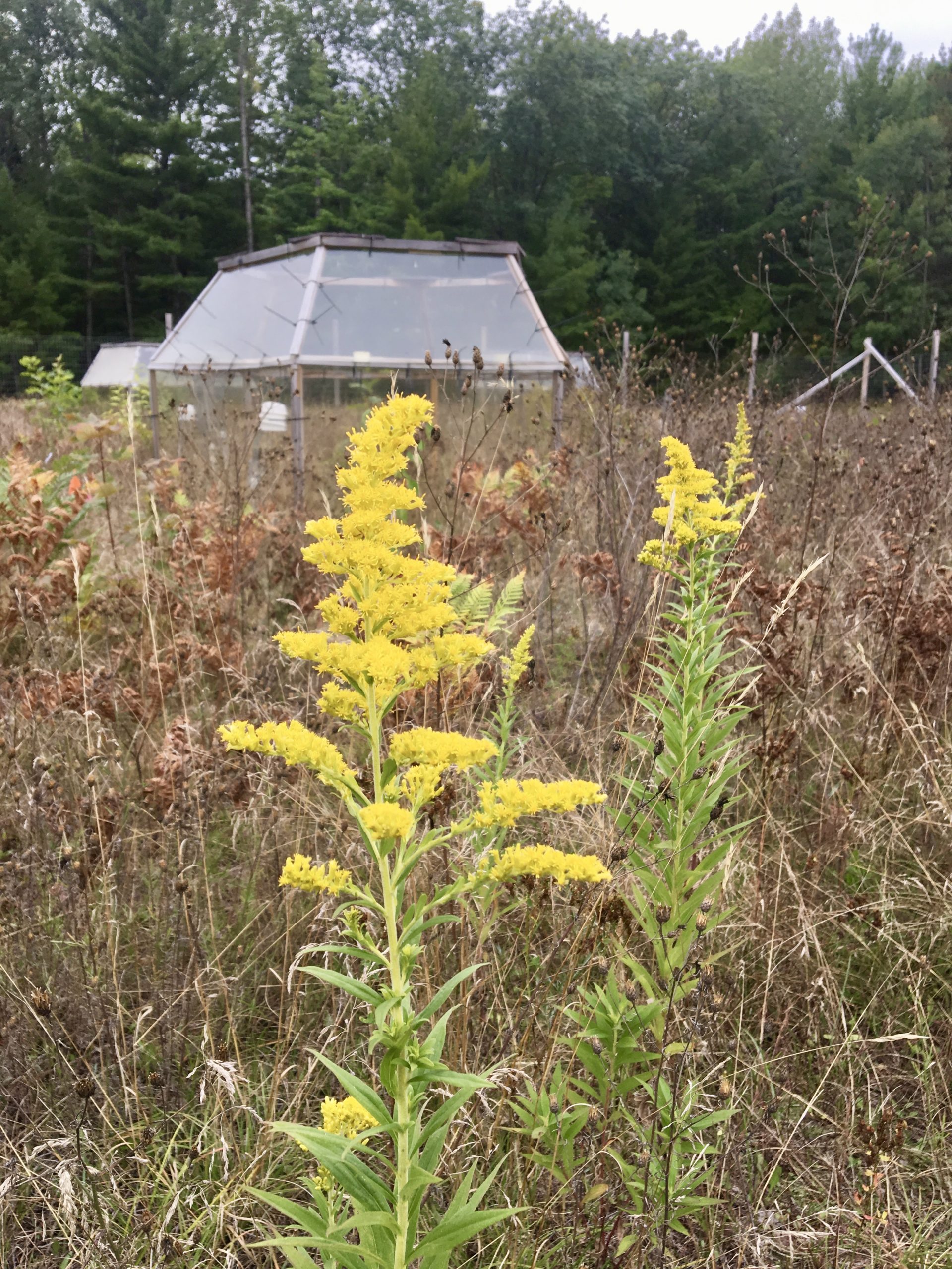
Tall goldenrod plants flowering in one of the ambient condition plots.

As you step into a warm greenhouse, you can feel how the glass has captured the sun’s heat inside. Now imagine that same warmth spreading across the entire planet due to increased greenhouse gas emissions. Climate scientists predict that by the year 2100, Earth’s average temperature could increase by as much as 3°C because of climate change. That might sound small, but even a few degrees matter a lot.

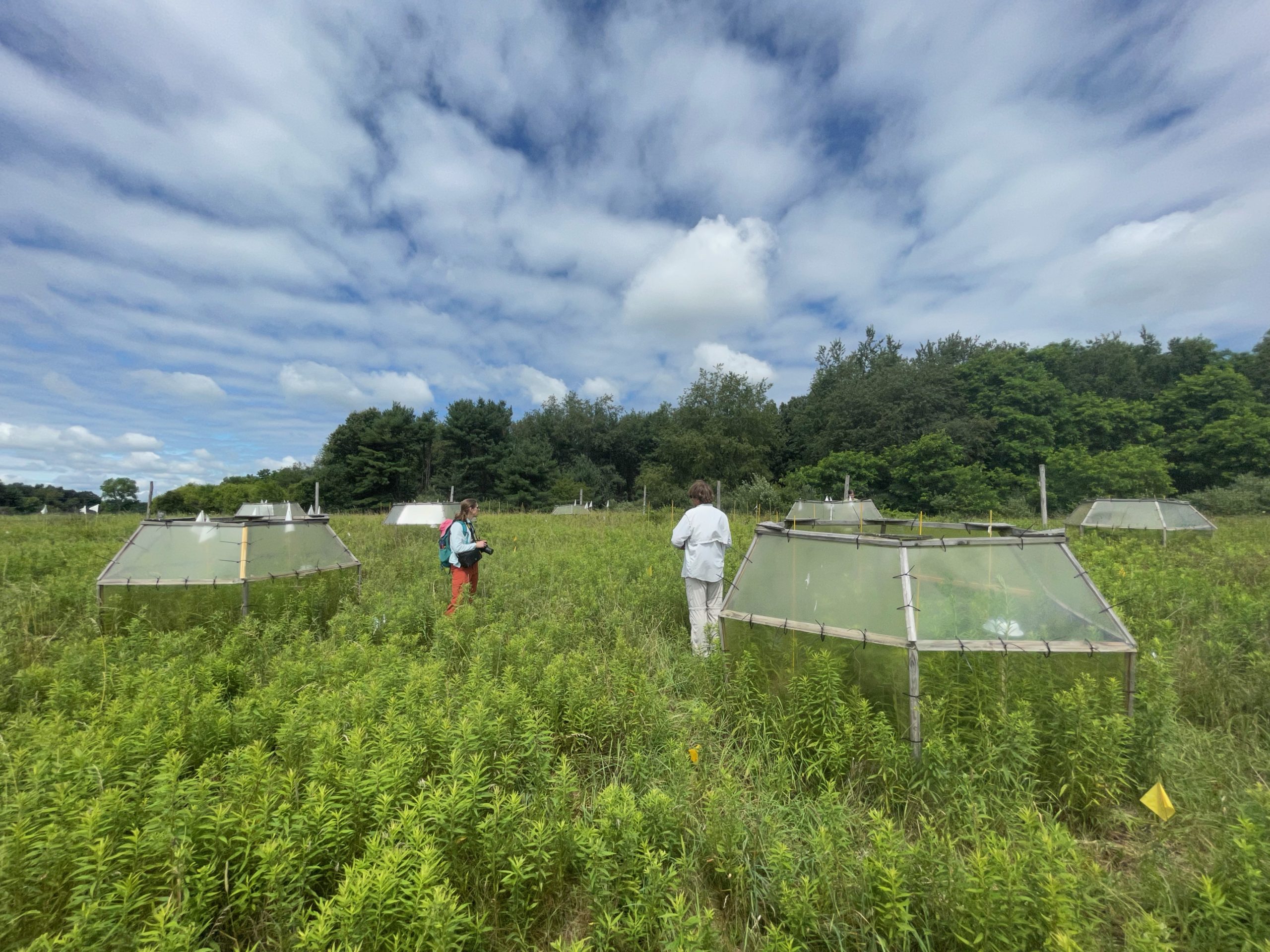
At the Kellogg Biological Station in southwest Michigan, a group of researchers wanted to know how climate warming will affect plant communities. To find out, they created what they call “mini time machines” using open-top chambers. These chambers are clear, hexagonal-shaped structures that trap heat and make the air inside warmer – just like a greenhouse. The chambers still allow for natural levels of precipitation, air flow, and insects to enter through their open tops. By comparing plant communities grown in these warmed conditionswith chambers, to ambient conditions without the chambers, scientists can see how rising temperatures might impact the plants in the future. Understanding these changes can help us prepare for a future where the climate is different from what we know today.

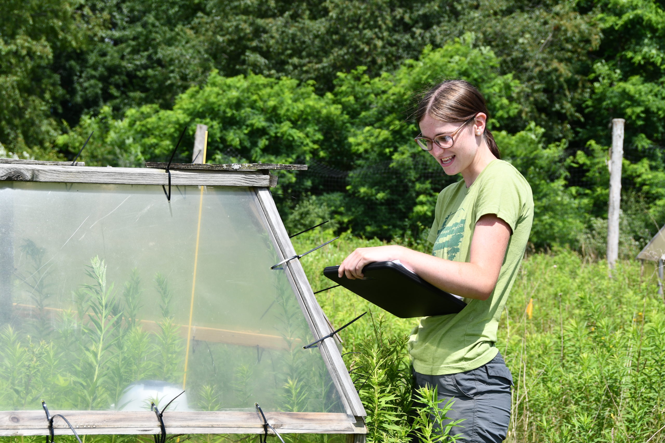
A scientist collecting data outside an open-top chamber.

The scientists working in the open-top chambers were at multiple stages in their careers. Moriah is a graduate student who became fascinated with plants when she first learned how to identify different species. Instead of looking at plants as all one patch of green, she could then notice all the diversity and the different roles they play in an ecosystem. Mark is a lab technician working with Moriah. He is interested in how plants will respond to warmer climates because it gives a glimpse of the world his grandchildren will see.

When Moriah and Mark started, they were joined by a few other scientists: Kara, another graduate student, and Emily, an undergraduate student. The open-top chambers had already been out in the field for five years. The field was growing with a diverse mix of plants common in the area. Together, they observed that plants growing in the warmed conditions inside the chambers seemed to be taller than those growing in the ambient conditions outside the chambers.

To collect some data to back up their observation, the team began with one species, tall goldenrod. This is a wildflower species with a bright yellow flower, and it is one of the most common species at this location. They wanted to see how goldenrod growth differed in warmed and ambient conditions. When temperatures rise, some plants grow faster and taller to compete for sunlight, but this takes a lot of energy. That means plants have less energy for survival, making seeds, or defending against herbivores, like insects. The researchers predicted that goldenrod inside the chambers would be taller, but would also have fewer stems and plants because they were putting their energy into growing tall instead of making more plants.

Open-topped chambers at the Kellogg Biological Station.

To test their ideas, the team measured goldenrod height with meter sticks and counted the number of goldenrod stems in each plot, called abundance. Their experiment had 30 plots. Half of the plots had open-top chambers, and half did not. That gave them 15 replicates of each treatment. Each plot is 1 meter x 1 meter. 

Featured Scientists: Mark Hammond (he/him), Moriah Young (she/hers), Kara Dobson (she/hers), and Emily Parker (she/hers) from the Kellogg Biological Station Long Term Ecological Research Program

Flesch–Kincaid Reading Grade Level = 9.3

Additional Resources:

  • The group of researchers featured in this activity work together at the Kellogg Biological Station, part of Michigan State University. Their lab is called the Spatial and Community Ecology Lab (SpaCE Lab). To learn more about their lab and work, students can visit their website or check out the Scientist Profiles associated with this activity.
  • Trevor Grabill produced a woodblock printed piece featuring the open-topped chamber experiment, titled What if it’s beautiful?. Along with the piece, they also produced a Zine that includes testimonials by the artist and scientists.

Missing species: the biodiversity of prairie remnants

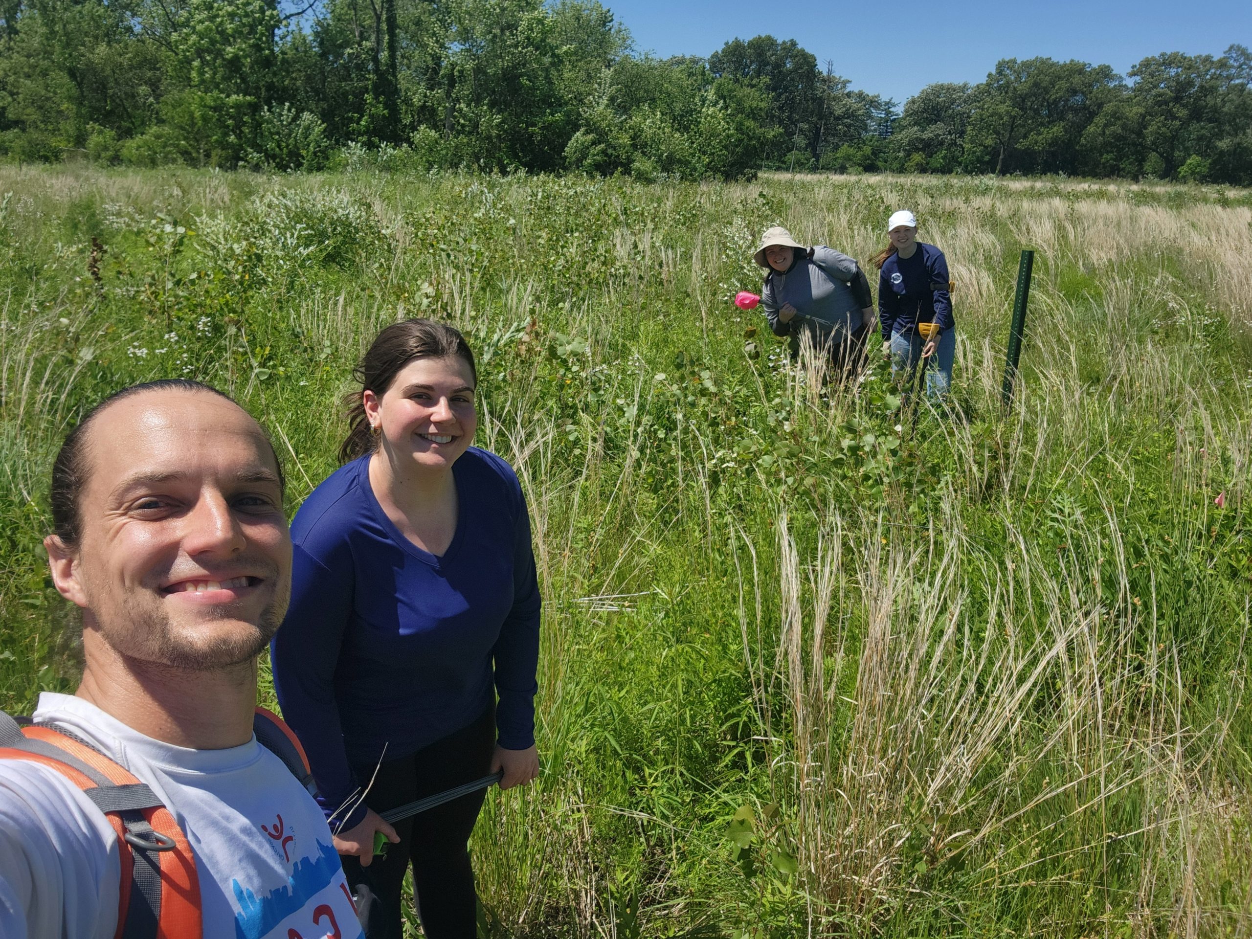
The scientist team visiting a prairie remnant field site.

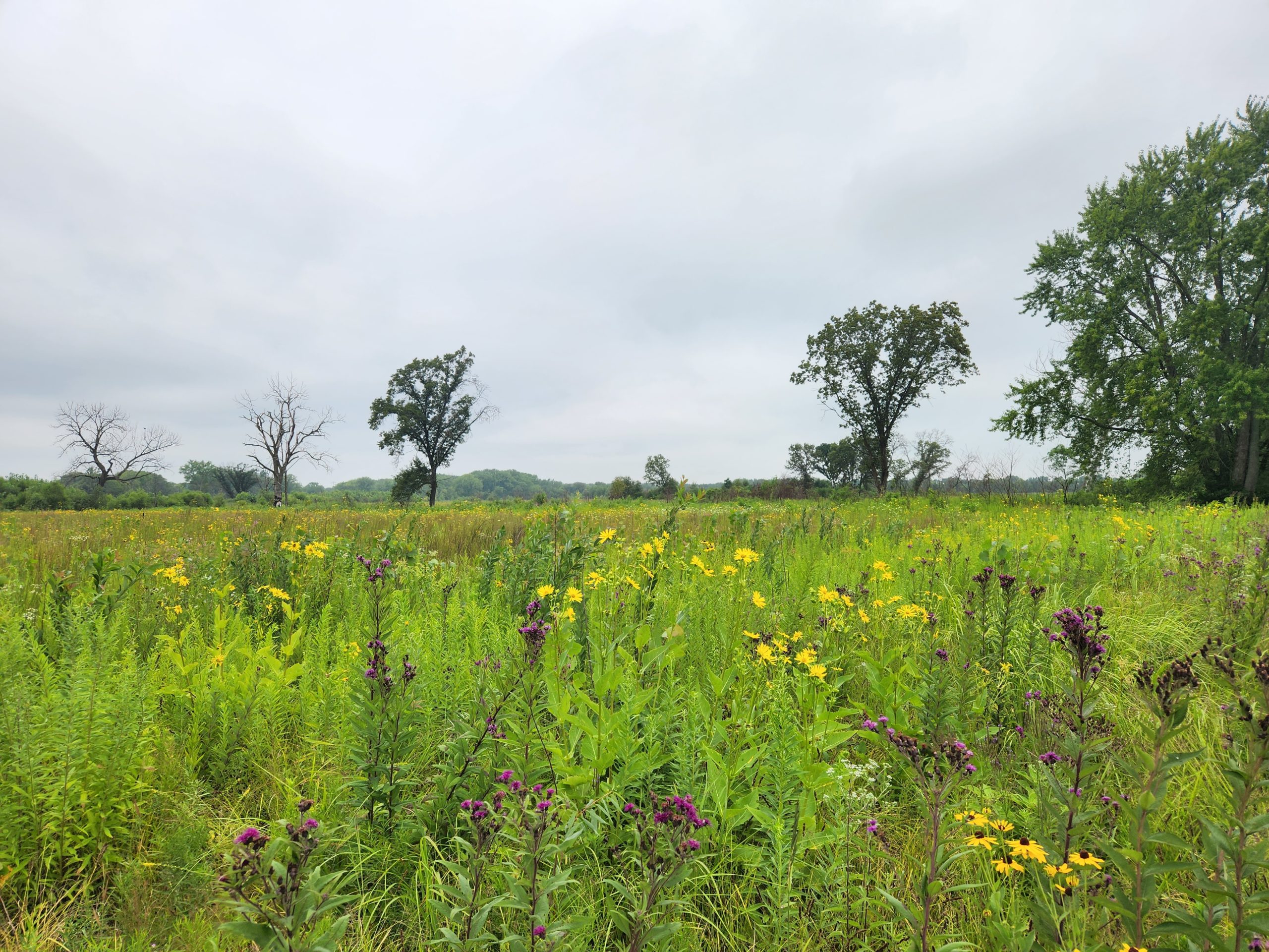
Illinois is called the “Prairie State.” Historically, 60% of the state was covered in different types of prairies, or open grassy landscapes with few trees. As far as the eye could see, fields were filled with colorful wildflowers, grasses, and all the species above and below ground that rely on them. However, today only 0.01% of the prairies remain across the whole state! These undisturbed areas are known as remnant prairies, and despite their small size, they are still home to a diverse community.

What happened to the rest of the prairies? Most were converted by people into agricultural fields to grow crops for food. The soils below prairies are rich in nutrients, and the agricultural lands in Illinois today provide food consumed by millions.

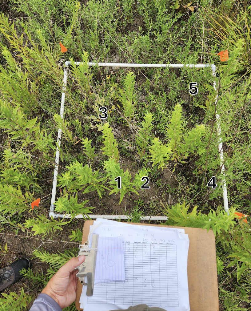
Researchers identifying plants in the field to document species richness. 

Nick is a land manager whose passion is prairies. In addition to protecting and studying remnant prairies, he creates restored prairies by planting prairie plants back into agricultural areas where they were historically found. However, Nick and other land managers are finding something surprising – the restored prairies do not look like the remnant prairies. He noticed that some of the native plants come back and thrive in the restored prairies, while others do not. 

To investigate these missing species, Nick partnered with a local scientist, Mike. Mike grew up in rural Michigan and has always been fascinated with biodiversity. He is passionate about bringing back missing species, because he knows even just one missing plant can have a cascading effect through an ecosystem. For example, wild lupine plants are a key food source for the endangered Karner blue butterfly. When prairie restorations have higher diversity, we’re more likely to benefit other species.  

Nick and Mike want to figure out why some species re-establish and others do not. They thought the key might lie belowground. From Mike’s past research, he knew that many prairie plants species form beneficial relationships with microbes belowground, called mutualisms. Could the root of the problem be explained by what is happening below ground? If these mutualist partners are missing in the soil, some plant species may not be able to survive.

One mutualist in prairies is called arbuscular mycorrhizal fungi, or AMF. Plants supply these fungi with sugars from photosynthesis. AMF help plant roots gather nutrients and water from the soil. AMF are common in prairie soils, but are often missing from soil that has been used for agriculture. Agriculture removes AMF in several ways. Tractors till the soil, disturbing the fungi below ground. Chemicals may be sprayed to kill harmful microbes, but these chemicals can also kill beneficial fungi, like AMF.

Nick chose an experimental site that was historically a sandy prairie, but had been used as a farm more recently. He used AMF originating from local remnant sand prairies to add to the experimental plots. Nick used a seed spreader to launch the AMF along the base of the plants. He set up three treatments that differed in how much AMF was applied: 1) a low level of AMF, 2) a high level of AMF, and 3) a control where no AMF was added. This setup was repeated 5 times in experimental blocks, or similar rectangular plots. 

After the growing season, Mike and his lab identified the plant species in each block. To help out, Jeremy joined Mike’s lab after finishing graduate school. He was a good fit because he had been working with similar data. Jeremy used the full dataset to calculate species richness, or the number of different plant species in each block. 

Featured Scientists: Mike Grillo and Jeremy Davis from Loyola University-Chicago and Nick Budde from the Forest Preserve District of Will County, Illinois. Written with Kerrie Rovito and Katarina Alvarado from Chicago Public Schools. Funding from the Walder Foundation.

Flesch–Kincaid Reading Grade Level = 8.8

Additional Teacher Resources:

If you would like to show students a remnant prairie that is close to where the scientists collected their data, you can see a video here.

You can see a video of Kankakee Sands, the area where the data were collected, here.

Videos about mycorrhizal fungi:

Superior watersheds: investigating stream health

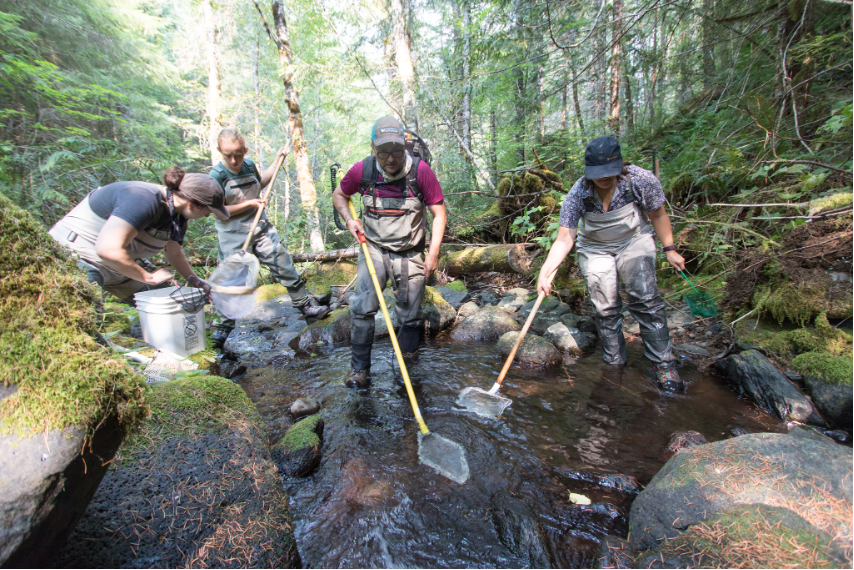
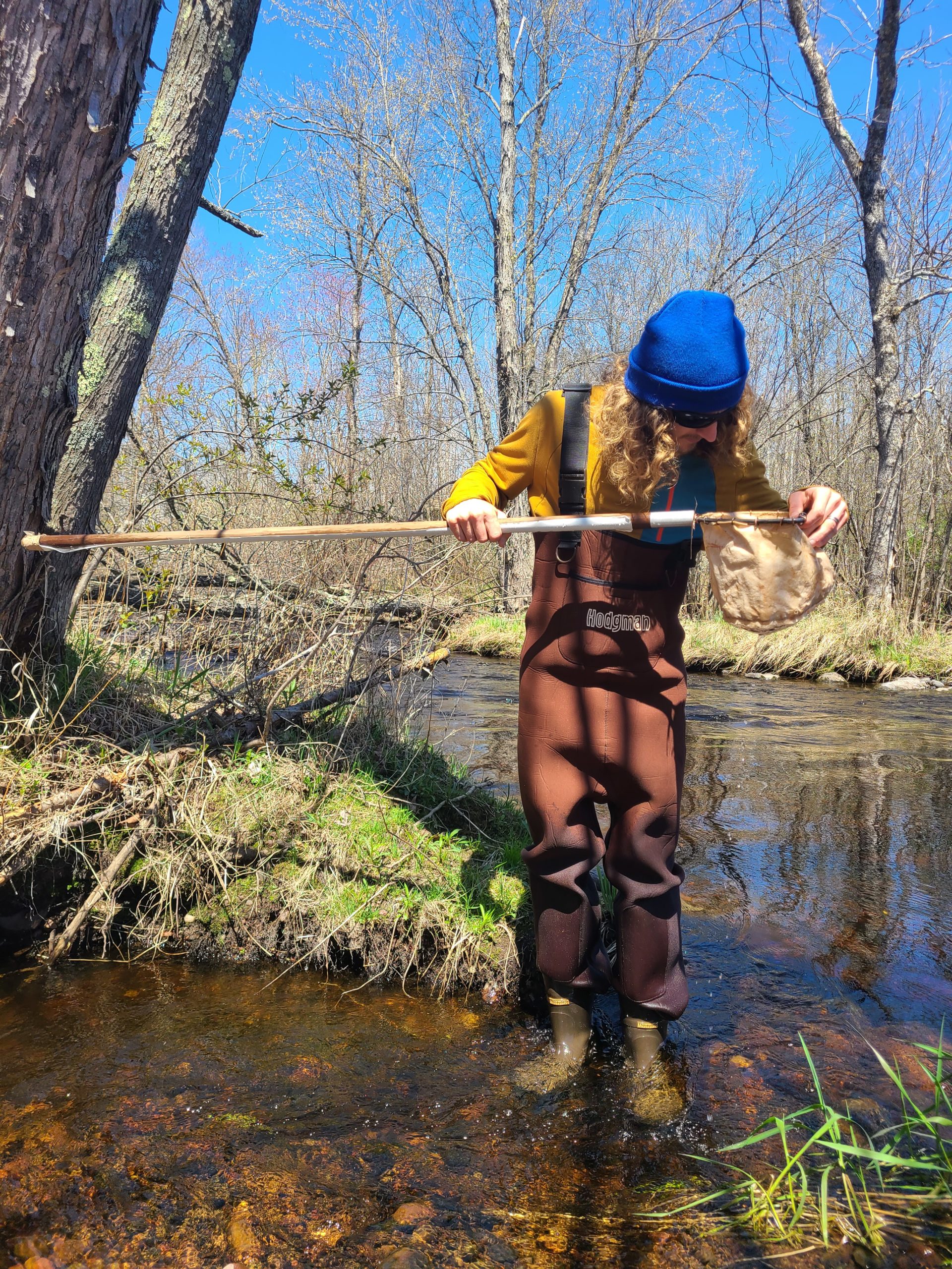
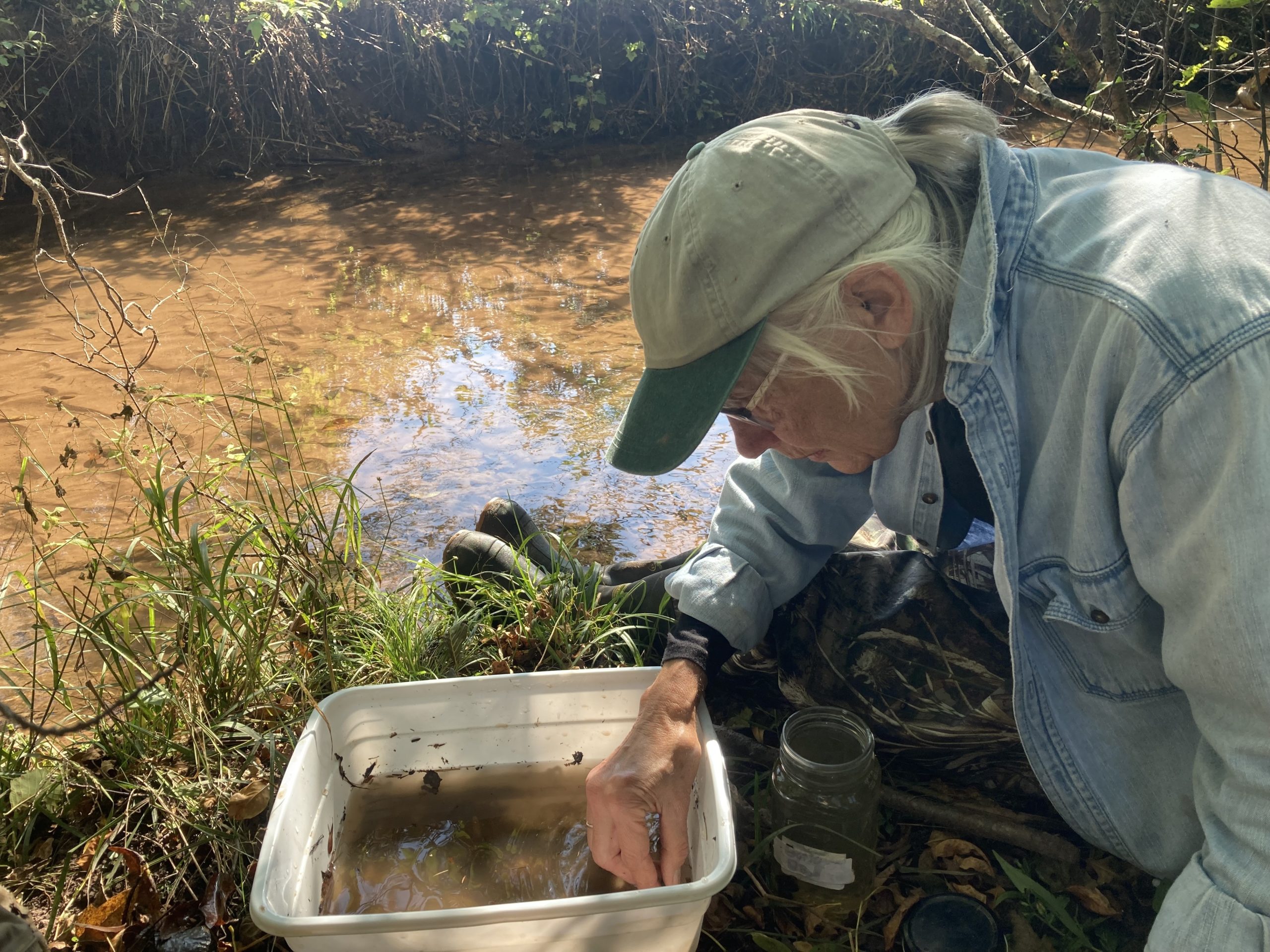
Will sampling macroinvertebrates from a stream using a D net.

Fresh water is one of our most important natural resources and an essential daily need for all people. Ten percent of the world’s freshwater is in Lake Superior. It is the largest lake in the world by surface area. It is also one of the cleanest, clearest, and coldest lakes in the United States. 

Watersheds are the network of rivers and streams, called tributaries, that flow into a single point and empty into a larger body of water. The water at the end of a watershed therefore reflects all the changes that happened across a large area. Thousands of tributaries flow through forests, wetlands, and farmland before reaching Lake Superior. These tributaries carry soil, nutrients, and any pollution from the land into the lake.

For a long time, people living near Lake Superior assumed that the tributaries had good water quality, but they didn’t have data to support this. In 2002, some residents living along the lake’s southern shore in Wisconsin came together to monitor the health of local tributaries themselves. They were already hearing how climate change, pollution, and land use were affecting water systems around the world. They formed an organization, now called Superior Rivers Watershed Association (SRWA) to collect long-term data so they could track changes in local tributaries.

SRWA volunteer sorting through macroinvertebrates from a stream sample.

Today, over 20 years later, SRWA has an established monitoring program. Members train volunteers to visit streams and rivers to collect data. Through these volunteers, SRWA has data on over 50 tributaries in the Lake Superior watershed. They collect data on both the water chemistry of the tributaries, as well as the life they find there. This helps them understand how water conditions affect organisms. 

Every spring and fall, volunteers visit their sites and sample macroinvertebrates, or small organisms that spend most or all their lives living on the stream bottoms. Many are larvae for insects you might know, such as dragonflies. After collecting samples, the volunteers identify each type of macroinvertebrate.

Each species has a different tolerance for stress, such as pollution, changes in temperature, low oxygen, or flooding. So, along with their biological data SRWA also collects data such as temperature, the amount of oxygen available in the water, and turbidity, or the amount of sediment in the water. Some species are indicators of good water quality because they need very clear, cold water, with a lot of oxygen, while others can survive in dirtier or harsher conditions. By seeing which macroinvertebrates live in each stream, scientists can learn about the health of the water.

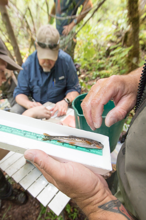
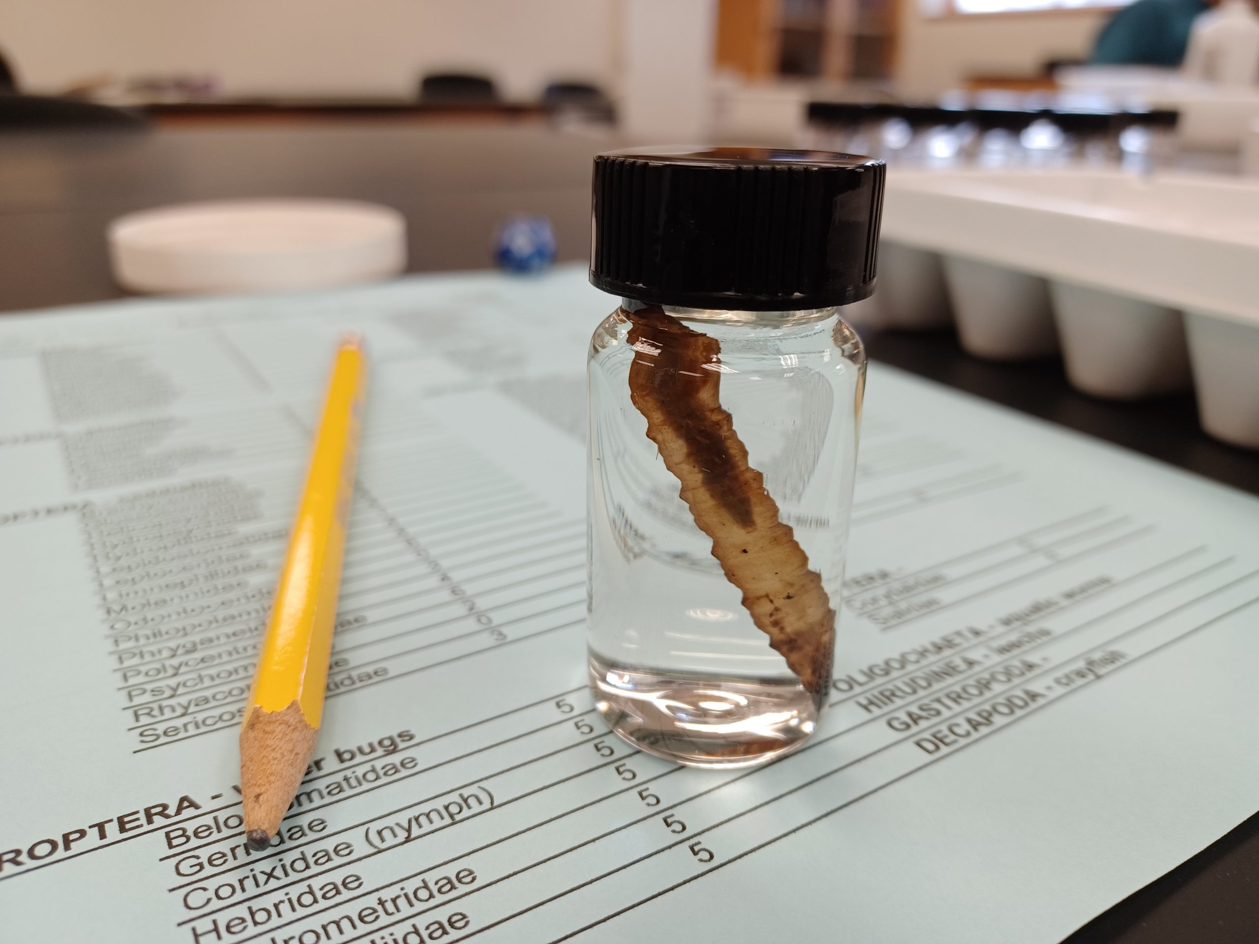
A macro invertebrate preserved for identification in the lab.

Two scientists, Will and Emma, are now analyzing over 20 years of volunteer data to identify trends and patterns. They want to see whether the water quality variables of temperature, dissolved oxygen, and turbidity affect the types of macroinvertebrates that can live in the tributaries. If there are a lot of sensitive indicator species in the sample, that is a good sign because it means the water quality is high. If they only find tolerant species, the water quality is likely poor, because indicator species were unable to survive in the environmental conditions at that site.

To do so, they use a tool called the Hilsenhoff Biotic Index. This index looks at which macroinvertebrates are present and how tolerant they are to pollution. HBI uses the living organisms that live at a site to provide an assessment of stream health over time, unlike chemical water tests which provide a snapshot of conditions at the time of testing. The index assigns a number from 1 to 10 based on the number and type of species in the sample. Lower numbers mean excellent water quality, and higher numbers mean poor water quality. 

Featured Scientists: Emma Holtan and Will Kendall with community volunteers from Superior Rivers Watershed Association. Written with: Andrea Pokrzywinski from Ashland High School.

Flesch–Kincaid Reading Grade Level = 10.8

Additional Teacher Resources:

Macroinvertebrate sampling is a common way to assess stream health in many regions. There are additional lesson plans and educational resources that you can use to supplement or expand on this Data Nugget activity. Andrea, a local teacher, works with SRWA to bring watershed monitoring into the classroom. She has put together a webpage with additional resources that she uses with her students.

On this webpage you will find:

  • Information on how to calculate the Hilsenhoff Biotic Index
  • Images and identification of common stream macroinvertebrates and their classification on the gradient from sensitive to tolerant
  • Stream sampling data sheets
  • Additional stream monitoring community science initiatives and programs with educational resources

Tiny but mighty: leaf miners take on aspen trees

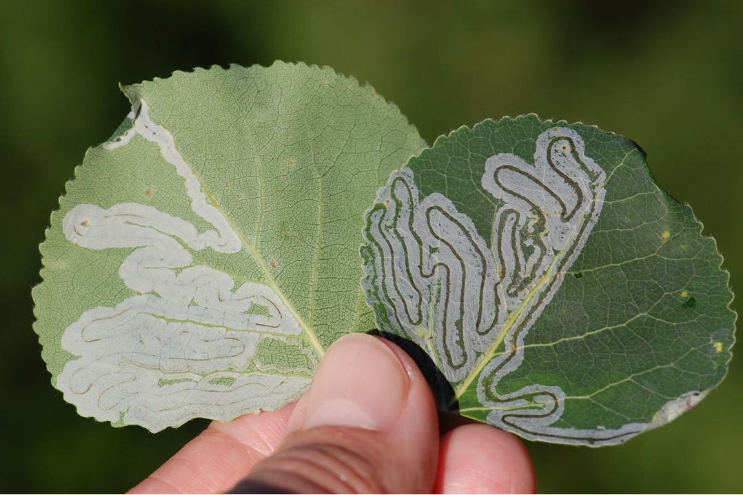
Leaf mining trails on the back (left) and front (right) of aspen leaves. Photo Credit: D. Wagner.

Caterpillars might look small, but can they actually be harmful?  Yes, if there are enough of them! Aspen leaf miners are moths as adults, but before that, aspen leaf miner caterpillars are incredible herbivores. In the spring, they lay their eggs on the surface of leaves, and they sink into the outer cell layer. When they hatch, the caterpillars quickly get to work. Using their blade-like mouth parts, they slash through the surface cell layer and drink the contents that are released. They leave a trail of silver, damaged cells in their path.

In recent years, aspen leaf miners have been increasing in numbers in Alaska and Canada. Aspen trees are an important component of the boreal forest, providing nutritious food for wildlife, supporting a diverse ecosystem, and capturing carbon dioxide (CO2) from the atmosphere at a high rate. Jenifer and Diane are two plant biologists who want to know if the aspen leaf miners are affecting leaves’ ability to do their job. Trees rely on their leaves to capture light energy for photosynthesis. During this process, cells convert CO2 gas from the atmosphere into sugar. Gases enter and leave through pores called stomata – CO2 comes in, and water vapor leaves. 

To avoid excessive water loss, leaves carefully control when the stomata are open. Stomata are surrounded by two sausage-shaped cells, called guard cells. The default position keeps the stomata closed. Different signals can cue the guard cells to open, but if too much water escapes, the stomata will close up again. 

In aspen trees, the guard cells are only on the bottom of the leaf. Jenifer and Diane suspected that leaf miners on the bottom side of the leaf would be destroying guard cells as they feed. They thought that if guard cells are no longer able to function properly, they would get stuck in the default closed position. This would limit photosynthesis because they would no longer be able to take in CO2 or let out water vapor.

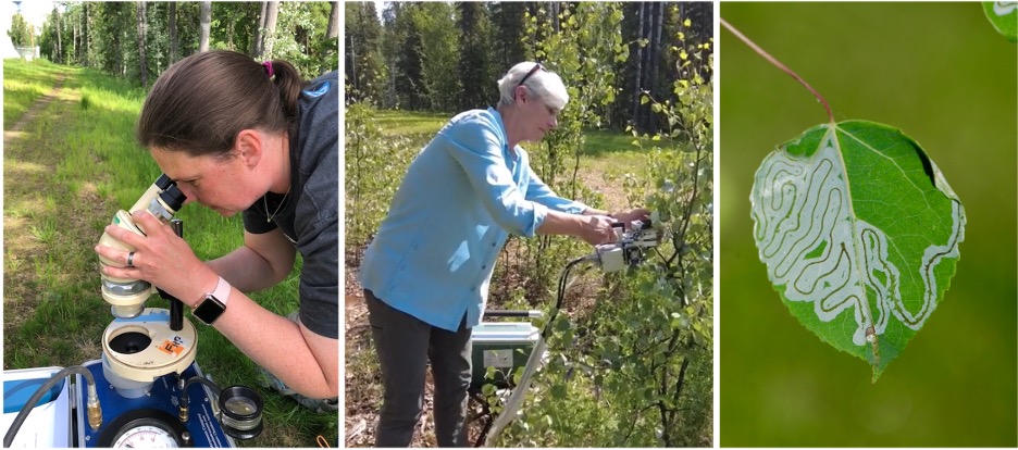
Left and middle: Diane and Jenifer taking measurements in the field; Right: a mined aspen leaf. Photo credits left to right: D. Wagner, D. Kind, D. Wagner.

To test their idea, Jenifer and Diane set up an experiment on the University of Alaska campus in Fairbanks. Jenifer and Diane let leaf miners lay eggs on leaves, like normal. Each caterpillar is so small that it stays on a single leaf side to eat. Jenifer and Diane removed eggs and marked about 10 leaves on each of 14 aspen trees. They randomly assigned each leaf to one of three treatments by removing the leaf miner eggs from either the top, bottom, or both sides of the leaves. To remove eggs from leaves, they wore magnifying headsets, just as a jeweler might wear, and carefully scraped each tiny egg off the leaf using a sharp probe. By doing so, they had leaves that were 1) mined on the bottom surface only, 2) mined on the top surface only, and 3) unmined (control) leaves. 

After the leaf miner caterpillars were finished feeding for the season, Jenifer and Diane came back to assess the damage. To understand the effect of the leaf mining damage on the leaves, they measured the photosynthesis and stomatal conductance of water vapor in the different treatments. To do this, they used a special piece of equipment called a portable infrared gas analyzer. The analyzer has two chambers – one that can be clamped onto a single leaf and one that is a control with no leaf. Gas is pumped through both chambers, and the gas concentrations from the leaf and the control are recorded and compared. The difference in CO2 concentration between the chambers is used to calculate the rate that CO2 is taken in by the leaf from photosynthesis. The difference in water vapor is used to measure how easily water vapor is passing out of the leaf through the stomata. 

Jenifer and Diane predicted that if the stomata are stuck closed, less CO2 would be taken from the atmosphere and less water vapor would be lost from the stomata. In other words, leaves with leaf miners on the bottom would have lower photosynthesis rates and decreased stomatal conductance of water vapor compared to the other treatments.

Featured scientists: Jenifer Wheeler (she/her) and Diane Wagner (she/her) from the University of Alaska Fairbanks. Written with Denise Kind (she/her).

Flesch–Kincaid Reading Grade Level = 9.3

Additional Teacher Resources:

There are short videos with background information on the study of aspen leaf miners in Alaska:

A scientific journal article about this research project: https://doi.org/10.1093/treephys/tpz109. Access the pdf here.

An additional educational module on the effects of the aspen leaf miners is available through the AKDatUM website.

The original data file can be found on the Bonanza Creek Long Term Ecological Research website, in the Data Catalog. Under Title, search for “leaf miner feeding damage”. There are many additional leaf physiology variables included in the data set. 

Live fast, die young?

Fast living snake (grey checked)
Slow living snake (dark with yellow stripe)
The two garter snake ecotypes – Fast living snake with grey checked pattern, and slow living snake with dark with yellow stripe.

Garter snakes are a common sight across North America, but one small species in Northern California has helped scientists learn a lot about how animals adapt to their environment. Since 1972, a long lineage of scientists has studied these snakes and passed their data down through generations. This long-term dataset allows scientists to ask questions about how replicate populations change over time.

These garter snakes live in two very different types of habitats. Some populations live along lakeshores at low elevations. These areas have rocky shorelines, warmer temperatures, and steady access to water and food like small fish and frogs. However, these snakes also face more predators. Other populations live in high-elevation mountain meadows. These habitats are cooler and covered in grass. Water and food are not always available and can change each year depending on snow and rain. Because these habitats are so different, the snakes in each place experience different challenges.

Over time, these differences have led to the evolution of two distinct ecotypes. Ecotypes are groups within a species that have adapted to their local environment. The lakeshore and meadow snakes differ in both their physical traits and their genetics. They also differ in how they grow, reproduce, and survive—traits known as life history strategies.

Life history strategies are often described along a spectrum from “fast” to “slow.” Lakeshore snakes have a “fast” life history. They grow quickly, reach adulthood sooner, are larger at adulthood, and produce larger and more frequent litters of offspring. In contrast, meadow snakes have a “slow” life history. They grow more slowly, reach adulthood later, have a smaller body size, and have fewer, less frequent litters.

Kaitlyn became interested in these snakes after a surprising start to her career. Interested in reptiles since childhood, she originally moved to Texas to join a lab that was studying turtles. Unfortunately, only a few weeks in, the grant money supporting her position fell through – right after she moved from Wisconsin to Texas! Luckily, another researcher invited her to join a lab studying snakes. After earning her Master’s degree, Kaitlyn continued this work during her PhD with her collaborator, Anne.

Kaitlyn and Anne wanted to understand how these snake populations are surviving today, especially after years of severe drought in California. They wondered if survival rates had changed over time and whether snakes in lakeshore and meadow habitats survived differently.

Scientists standing on a rocky lakeshore looking for snakes.
Flipping rocks and reaching into stinging nettle at Lakeshore sites.

To answer these questions, Anne and Kaitlyn wanted to take a fresh look at snake survival rates. They went out into the field to collect their own data, and compared their estimates to over 50 years of prior data collection. Both the historic and current data were collected using the method called capture-mark-recapture. In this method, researchers catch snakes, measure traits like size and weight, and give each snake a unique mark before releasing it back into the wild. If a snake is caught again later, scientists can track how it has grown. Not all snakes are recaptured. These data can be used to estimate survival rates, though some snakes may have moved away or avoided being caught.

Because it is hard to know the exact age of each snake, Kaitlyn grouped them into four age classes based on size: neonates (newborns), juvenilesyoung adults, and old adults. She then used statistical models to use her capture-mark-recapture dataset to estimate the probability of survival for each group. Kaitlyn predicted that meadow snakes, with their “slow” life history strategy, would have higher survival rates than lakeshore snakes. She also expected this difference to be greatest in young snakes.

Featured scientists: Kaitlyn Holden (she/her) and Anne Bronikowski (she/her) from Michigan State University

Flesch–Kincaid Reading Grade Level = 9.4

Additional Teacher Resources:

  • Scientist profile: Anne Bronikowski has a scientist profile to supplement this activity. Have students read more about her research, personal life, and career advice as a way to share contemporary scientist role models with students!
  • You can learn more about the IISAGE (Integration Initiative: Sex, Aging, Genomics, and Evolution) project here. This initiative is a collaborative effort to learn more about the mechanisms of sex-specific differences in aging and features research with a variety of organisms.
  • Visit this page for additional scientist profiles and Data Nuggets featuring IISAGE research.

The chromosome advantage: Lifespan differences across sexes

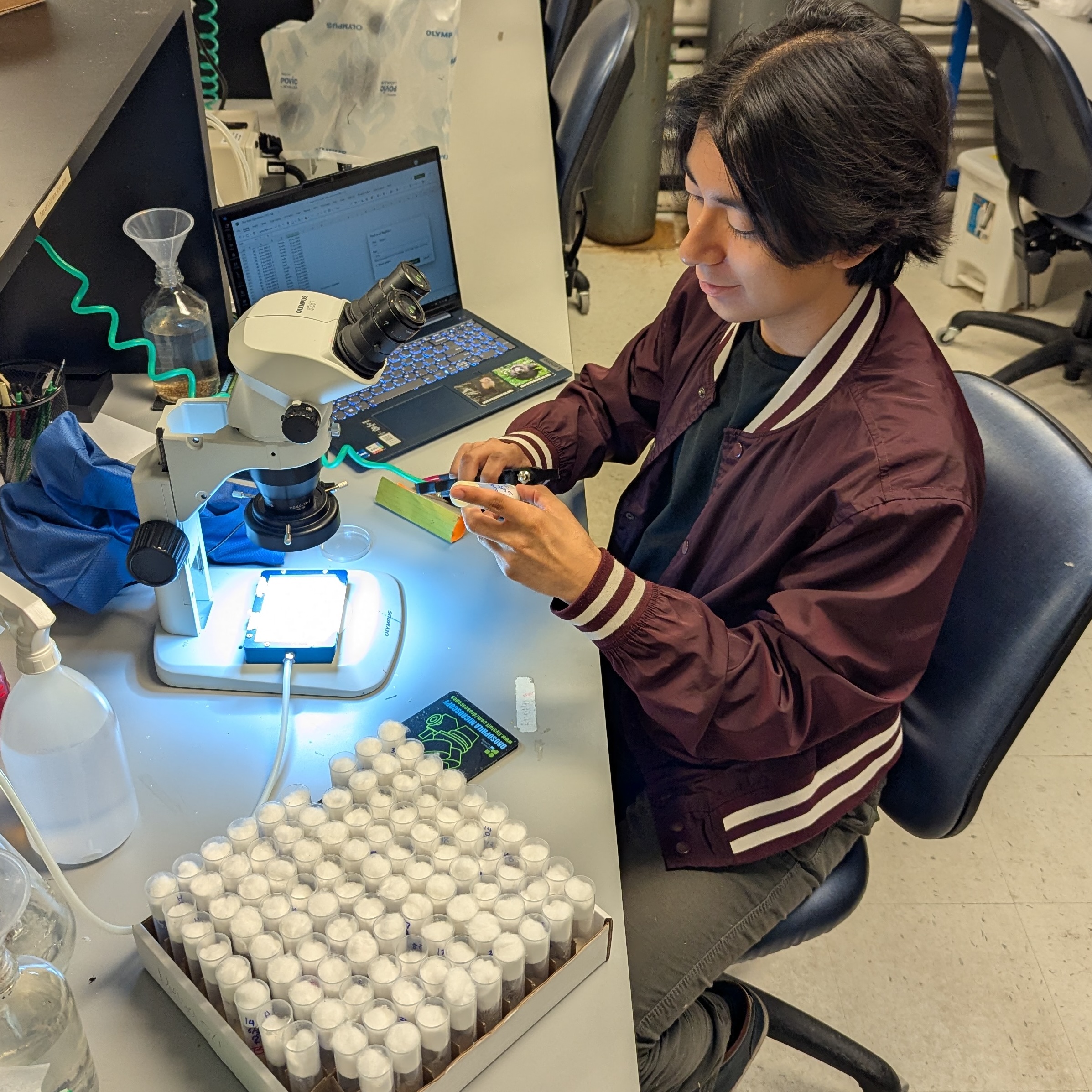
Nicole Riddle looking at fruit flies under the microscope

The activities are as follows:

Many factors affect lifespan, or how long an organism lives. Different species, and individuals within a species, will all live to different ages. Across species, things like body size, rate of metabolism, and genetics can all come into play. For example, larger animals tend to live longer than smaller organisms. Within a species, genetics and environmental conditions, such as being able to find food, the presence of predators, and disease, will also impact survival.

Scientists have also noticed that in many animal species, one sex tends to live longer than the other. Sometimes it is the males, and sometimes it is the females. Why might this be? To better understand aging differences across sexes, a group of scientists decided to work together. Each scientist studies a different species, so by combining their knowledge, they can look for patterns and see if there are consistent factors that are the cause.

Jamie Walters running DNA extractions in the lab.

Nicole and Jamie are two scientists in this group. Nicole studies fruit flies, while Jamie studies moths and butterflies. Even though fruit flies and moths are both insects, sex is determined differently. In most animals, biological sex is determined by specific chromosomes. These structures are inside cells and carry genetic information. Individuals usually have two sex chromosomes. Whether those two chromosomes are the same or different often determines whether their bodies develop as male or female.

In fruit flies, females have two of the same sex chromosomes (XX), while males have two different sex chromosomes (XY). In moths and butterflies, the pattern is reversed. Males have two of the same sex chromosomes (ZZ), while females have two different ones (ZW).

Nicole and Jamie wondered if having two different sex chromosomes might affect lifespan. When an individual has only one copy of a particular chromosome—like the X in XY males or the Z in ZW females—there is no second copy for the genes on that chromosome. If that single copy contains a harmful mutation or becomes damaged, the organism cannot rely on a second copy to make up for it. On the other hand, individuals with two of the same sex chromosomes (XX or ZZ) have a kind of “genetic backup”. This extra protection might reduce the risk of problems that could lead to an earlier death.

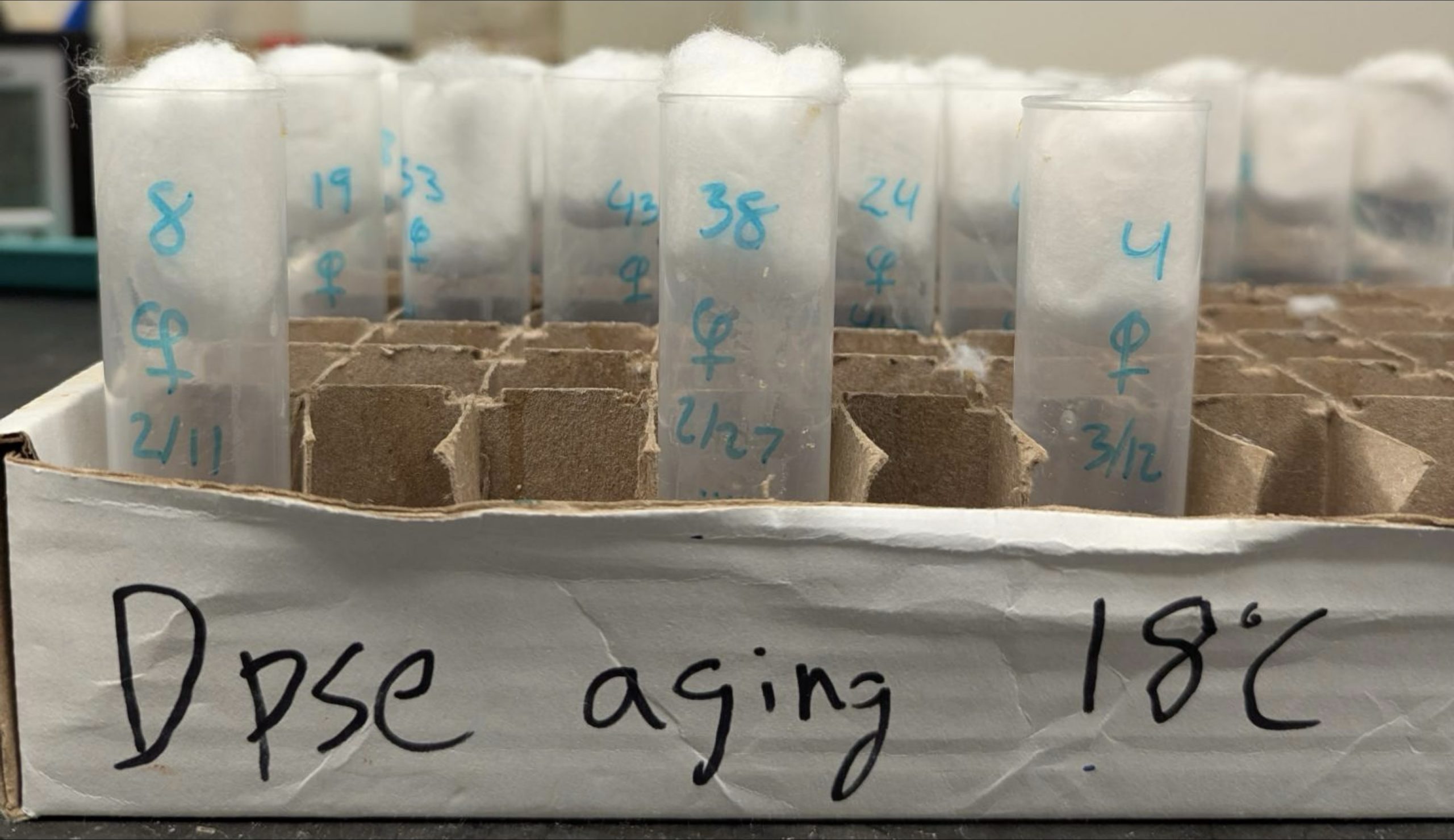
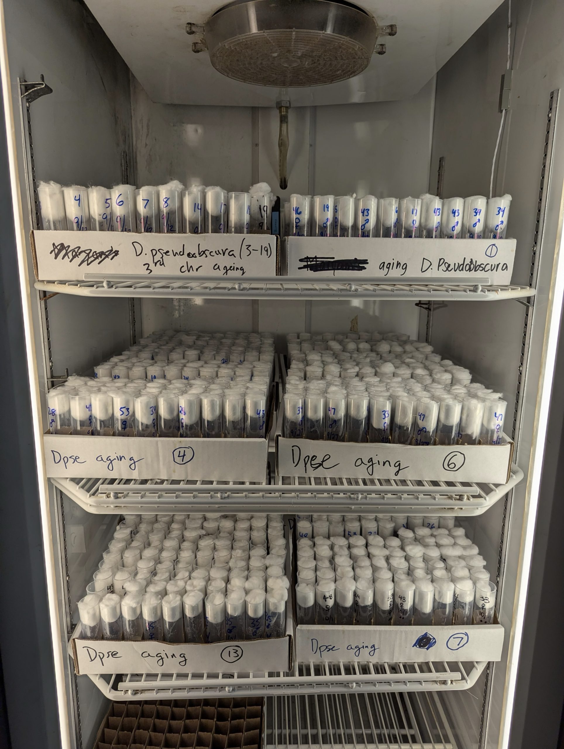
To test their idea about sex chromosomes and lifespan, Nicole and Jamie designed an experiment called a survival assay. A survival assay is a laboratory experiment in which scientists carefully track how long organisms live under controlled conditions. By keeping the environment consistent, scientists can focus on the specific factor they want to study.

Nicole works with fruit flies (left) and Jamie studies pantry moths (right). 
 
Plodia interpunctella female by Pekka Malinen, Luomus is licensed under CC BY-SA 4.0.

Nicole performed her survival assay with the fruit fly species, Drosophila melanogaster. Jamie worked with a pantry moth species called Plodia interpunctella. Both scientists already raise these species in their labs and carefully document the life cycles and age of each individual.

To set up their assays, Nicole and Jamie chose individuals that had emerged from the pupae stage around the same time. This step was important because they wanted to make sure all individuals had the same starting point. If some individuals had emerged a lot sooner, the results would not be accurate.

Nicole collected 100 female and 100 male fruit flies, and Jamie collected 60 male and 60 female moths. The insects were given plenty of food and kept in good environmental conditions, such as appropriate temperature and humidity. By reducing stress, they could better observe natural lifespan differences between males and females, rather than differences caused by harsh conditions.

Each day, Nicole and Jamie recorded how many males and females were still alive. This careful daily tracking allowed them to see how survival changed over time. The survival assay continued until the last individual had died. By the end of the experiment, Nicole and Jamie had detailed data showing how long males and females lived in each species. These results would help them test whether having two identical sex chromosomes—or two different ones—might influence lifespan.

Featured scientists: Nicole Riddle (she/her) from the University of Alabama at Birmingham and Jamie Walters (he/him) from the University of Kansas.

Flesch–Kincaid Reading Grade Level = 9.9

Additional Teacher Resources:

  • Scientist profiles: Nicole Riddle and Jamie Walters both have scientist profiles to supplement this activity. Have students read more about their research, personal lives, and advice they have as a way to share contemporary scientist role models with students!
  • You can learn more about the IISAGE (Integration Initiative: Sex, Aging, Genomics, and Evolution) project here. This initiative is a collaborative effort to learn more about the mechanisms of sex-specific differences in aging and features research with a variety of organisms.
  • Visit this page for additional scientist profiles and Data Nuggets featuring IISAGE research.

What wakes the squirrels?

An arctic ground squirrel checking out the scientists from inside a trap
An arctic ground squirrel checking out the scientists from inside a trap. Photo by Rachel Rigenhagen.

The activities are as follows:

The Arctic is home to a unique biome, known as tundra. Found at Earth’s northernmost region, the tundra ecosystem is defined by frozen land. Permafrost is a thick underground layer of organic matter, soil, rock, and ice that has been frozen for at least two full years. Each summer as the temperature warms, a thin upper layer of frozen soil thaws, refreezing again the following winter.

Although the tundra might be far away from where most people live, it is connected to the entire globe through the atmosphere. This means it is affected by climate change, just like other places on Earth. In the tundra, increasing temperatures are causing snow to melt and the top layer of permafrost to thaw earlier each year.

Arctic ground squirrels, also called siksik (pronounced shrick-shrick) in the Inuktitut language, are an important mammal species that call the tundra home. They hibernate for roughly eight months – the longest of any mammal in the world. As they hibernate, the snow and frozen permafrost insulate their burrows and protect them from severe cold. As the summer months approach, the squirrels emerge and move above ground. Their mating season begins immediately after hibernation ends. With only four months out of their burrows, they have to maximize their time! 

Cory is a scientist who lives in Colorado but travels to the Arctic to do research at Toolik Field Station. For over 25 years, Cory and his research team have been studying the ground squirrel populations. While at Toolik recently, Cory was surprised to discover that male and female ground squirrels were emerging from hibernation on different schedules. He is worried these mismatches could be due to climate change. 

Austin holding an arctic ground squirrel that has been tagged in front of an Arctic scene background.
Austin, a PhD student in Cory’s lab, releases an arctic ground squirrel that has been tagged. Photo by Rachel Rigenhagen.

This made Cory wonder how ground squirrels know when to come out of their burrow. He suspected that ground squirrels use cues from their environment, such as increasing temperatures, permafrost thaw levels, or the length of time they have been in hibernation. Some of these environmental cues, such as the timing of permafrost thawing, are affected by increased temperatures. Other cues are not affected by temperature, such as the length of time squirrels have been hibernating. If males and females are using different cues, this could be why they are coming out at different times.

To investigate his idea, Cory and his research team turned to data they have been collecting over time. Each year, the research team temporarily captures squirrels. They record each squirrel’s sex, give them a unique ID, and put collars on them before releasing them. The collars can detect light, which is used to know when the squirrels are above ground. For each squirrel, the team records the first date that light was detected after hibernation, called the emergence date. Cory used Julian dates, which start with January 1 as Day 1 and continue to count up by one for each day. 

Cory also looked at the data on snowmelt as a potential environmental cue that the squirrels were using. Each year Cory’s team installs cameras on tall towers so that they can use images to measure daily snow cover. When no snow was detected, they measured this as the snowmelt date. Using these two sources of data, they can look for any patterns in emergence dates and spring snow melt. 

Featured scientist: Cory Williams (he/him) from Colorado State University and Toolik Field Station. Written by Claire Gunder (she/they) and Rachel Rigenhagen (she/her), Avalon School, St. Paul, Minnesota.

Flesch–Kincaid Reading Grade Level = 8.7

Pollination matters

A Mexican petunia in the bagged self-pollination treatment.

The activities are as follows:

Pollination is one of nature’s most important processes. Without pollen moving from one plant to another, many plants would not be able to produce fruits or seeds. Without pollination, we wouldn’t have food like apples, strawberries, or even chocolate! But not all pollination works the same way. Some plants rely on pollinators like bees and butterflies, while others can reproduce without any help at all. Scientists are still exploring why plants have these different strategies.

As a science teacher, Cynthia is always looking for ways to bring real science into her classroom. To learn more about the work of scientists, she joined a summer research program. While there, she had the opportunity to design and carry out a study on pollination in a plant species, Mexican petunia.

Mexican petunias are a flowering plant found in gardens, parks, and wild spaces. They have bright purple flowers. This plant has two ways it can be pollinated, called pollination methods. First, insect pollinators visit and move pollen. When pollen is moved from one plant to another, this is called outcrossing. Second, these plants can self-pollinate, meaning pollen from a single flower can pollinate that same flower. 

Pollination methods make a big difference for plants. Outcrossing mixes the genetics of two different plants together, which creates new genetic combinations that may help offspring survive and thrive. In contrast, self-pollination means the genetics of the plant are the same as the parent plant and no new genetic combinations are made. Plants that use self-pollination don’t need to rely on pollinators, however many times the seeds they produce are not viable and are not able to grow. 

Cynthia predicted that outcrossing would produce the most fruits and seeds, and flowers that relied on self-pollination would produce fewer seeds. She designed a garden experiment where she could control how Mexican petunias were pollinated. To set up her study, she used four different treatments. 

Bagged – Cynthia put mesh bags around the petunia flowers. This prevents pollination from other plants, so this treatment shows whether flowers are able to successfully self-pollinate on their own.

Open pollination – Cynthia left these flowers open to visits from insects. These plants could be self-pollinated or outcrossed.

Self-pollinated by hand – Cynthia hand-pollinated these flowers using pollen from another flower on the same plant. This treatment shows whether the plant produces fruit when the flowers are self-pollinated by hand.

Outcrossed by hand – Cynthia hand-pollinated these flowers with pollen from a different Mexican petunia plant. These plants are all outcrossed.

Cynthia monitored the Mexican petunia plants in her four treatments for three weeks. She checked the flowers every few days to see which ones developed fruit. If a flower made a fruit, she counted the number of seeds per fruit. In the open pollination treatment, a few times the fruit opened and launched out its seeds before Cynthia could count them, meaning she could get fruit data from the flower, but not a seed count. At the end of her experiment, she had collected data on percent fruit development, or the chance of successful development of a fruit from a flower, and the number of seeds produced within those fruits, called seed count.

Featured scientist: Cynthia Nuñez from Florida International University

Flesch–Kincaid Reading Grade Level = 8.8