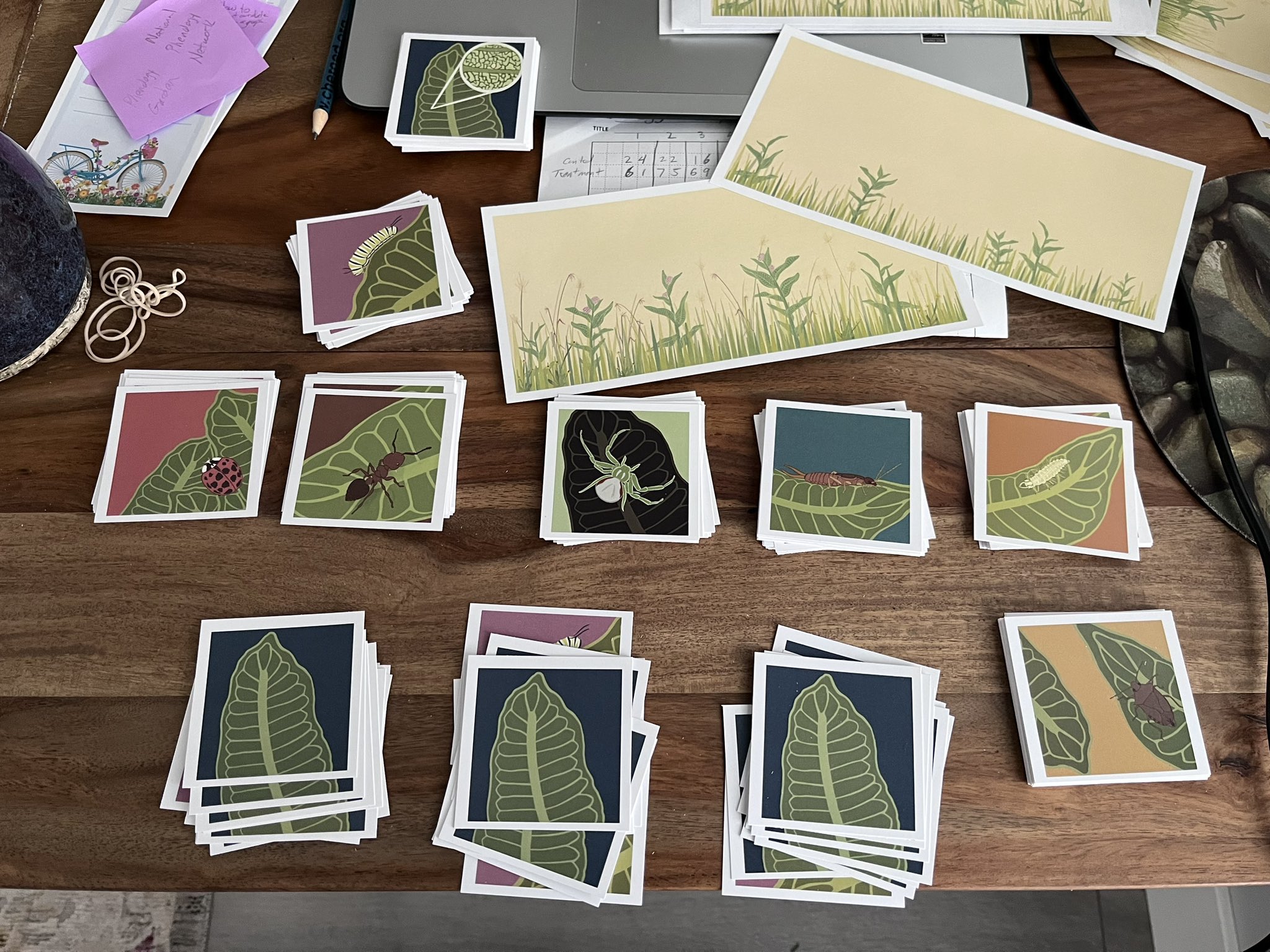
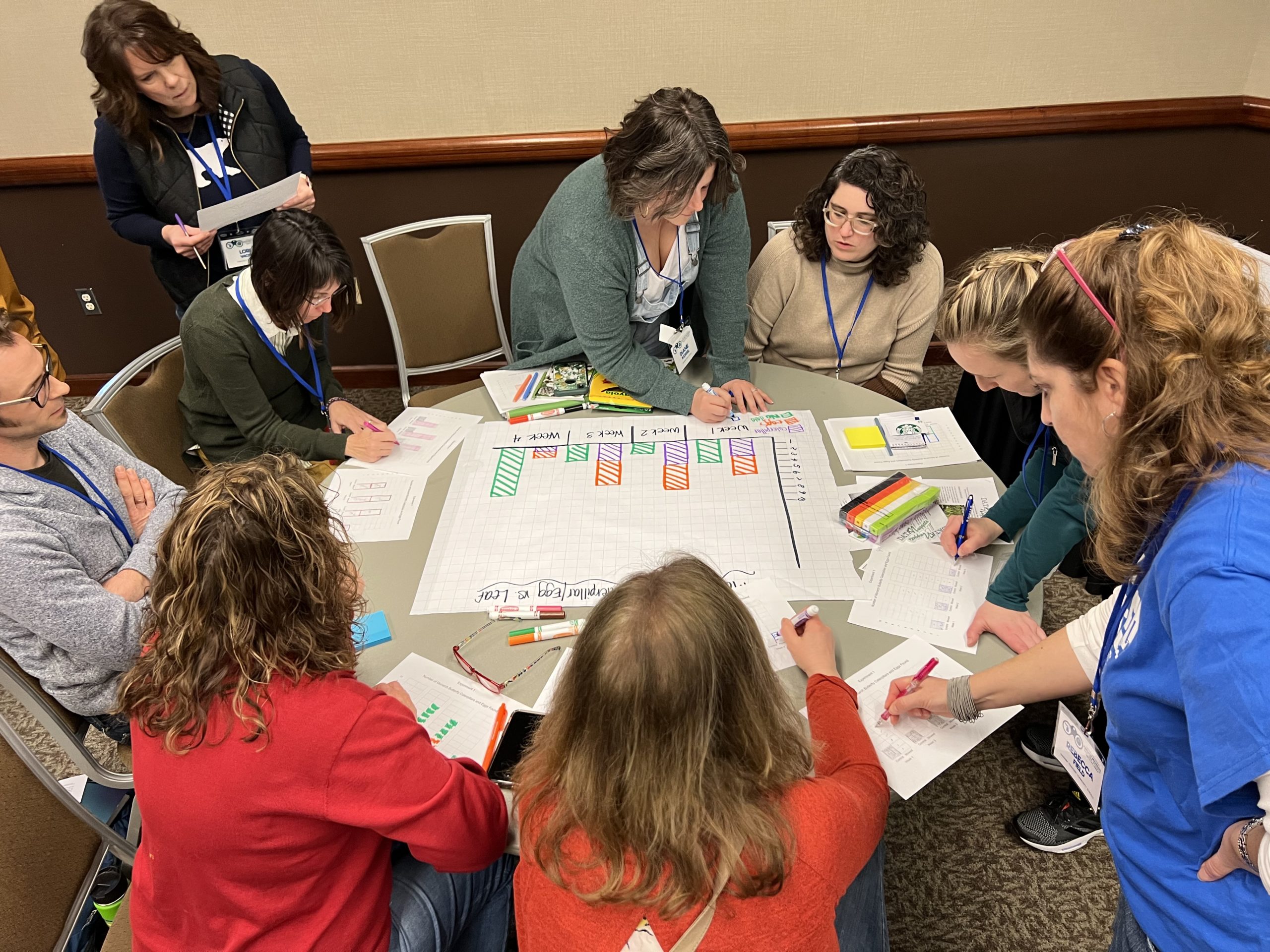
Getting to the roots of serpentine soils

Alexandria in the field observing the plants and soil.

When an organism grows in different environments, some traits change to fit the conditions. For example, if a houseplant is grown in the shade, it might grow to stretch out long and thin to reach as much light as possible. If that same plant were grown in the sun, it would grow thicker stems and more leaves that are not spread as far apart. This response to the environment helps plants grow in the different conditions they find themselves in.

Flexibility is especially important when a plant is living in a harsh environment. One such environment is serpentine soils. These soils are created from the weathering of the California state rock, Serpentinite. Serpentine soils have high amounts of toxic heavy metals, do not hold water well, and have low nutrient levels. Low levels of water and nutrients found in serpentine soils limit plant growth. In addition, a high level of heavy metals in serpentine soils can actually poison the plant with magnesium!

Combined, these qualities make it so that most types of plants are not able to grow on serpentine soils. However, some plant species have traits that help them tolerate these harsh conditions. Species that are able to live in serpentine soils, but can also grow in other environments, are called serpentine-indifferent.

Alexandria has been working with serpentine soils since 2011 when she was first introduced to them during an undergraduate research experience with her ecology professor. Alexandria was especially intrigued by this challenging environment and how organisms are able to thrive in it, even with the harsh characteristics.

Dot-seed plantain plants in the growth chamber.

To learn more, she started to read articles about previous research on plants that can only grow in serpentine soils. Alexandria learned that these plant species are generally smaller than closely related species. This was interesting, but she still had questions. She noticed the other experiments had compared plant size in different species, not within one species. She thought the next step would be to look at how plants that are the exact same species would respond to serpentine and non-serpentine soil environments. To explore this question, she would need to use serpentine-indifferent plant species because they can grow in serpentine soils and other soils.

Just as a houseplant grows differently in the sun or shade, plants grown in serpentine and non-serpentine soils might change to survive in their environment. Alexandria thought one of these changes could be happening in the roots. She decided to focus on plant roots because of their importance for plant survival and health. Roots are some of the first organs that many plants produce and anchor them to the ground. Throughout a plant’s life, the roots are essential because they bring nutrients to above-ground organs such as leaves. Because serpentine soils have fewer plant nutrients and are drier than non-serpentine soils, Alexandria thought that plants growing in serpentine soils may not invest as much into large root systems. She predicted plants growing in serpentine soils will have smaller roots than plants growing in non-serpentine soils.

To test her ideas, she studied the effects of soil type on a serpentine-indifferent plant species called Dot-seed plantain. She purchased seeds for her experiment from a local commercial seed company. About 5 seeds were planted in serpentine or non-serpentine soils in a growth chamber where growing conditions were kept the same. After the seedlings emerged, the plants were thinned so that there was one plant per pot. The only difference in the environment was the soil type. This allowed Alexandria to attribute any differences in root length to serpentine soils. At the end of her experiment, she pulled the plants out of the soil and measured the root lengths of plants in both treatments.

Featured scientist: Alexandria Igwe (she/her) from University of Miami

Flesch–Kincaid Reading Grade Level = 8.7

Additional resources related to this Data Nugget:

The topics described in this Data Nugget are similar to the published research in the following article:

  • Igwe, A.N. and Vannette, R.L. 2019. Bacterial communities differ between plant species and soil type, and differentially influence seedling establishment on serpentine soils. Plant Soil: 441: 423-437

There is a short video of Alexandria (Allie) sharing her research on serpentine soils.

There have been several news stories and blog posts about this research:

Mangroves on the move

mangrove in marsh
A black mangrove growing in the saltmarshes of northern Florida.

The activities are as follows:

All plants need nutrients to grow. Sometimes one nutrient is less abundant than others in a particular environment. This is called a limiting nutrient. If the limiting nutrient is given to the plant, the plant will grow in response. For example, if there is plenty of phosphorus, but very little nitrogen, then adding more phosphorus won’t help plants grow, but adding more nitrogen will. 

Saltmarshes are a common habitat along marine coastlines in North America. Saltmarsh plants get nutrients from both the soil and the seawater that comes in with the tides. In these areas, fertilizers from farms and lawns often end up in the water, adding lots of nutrients that become available to coastal plants. These fertilizers may contain the limiting nutrients that plants need, helping them grow faster and more densely.

One day while Candy, a scientist, was out in a saltmarsh in northern Florida, she noticed something that shouldn’t be there. There was a plant out of place. Normally, saltmarshes in that area are full of grasses and other small plants—there are no trees or woody shrubs. But the plant that Candy noticed was a mangrove. Mangroves are woody plants that can live in saltwater, but are usually only found in tropical places that are very warm. Candy thought the closest mangrove was miles away in the warmer southern parts of Florida. What was this little shrub doing so far from home? The more that Candy and her colleague Emily looked, the more mangroves they found in places they had not been before.

Candy and Emily wondered why mangroves were starting to pop up in northern Florida. Previous research has shown nitrogen and phosphorus are often the limiting nutrients in saltmarshes. They thought that fertilizers being washed into the ocean have made nitrogen or phosphorus available for mangroves, allowing them to grow in that area for the first time. So, Candy and Emily designed an experiment to figure out which nutrient was limiting for saltmarsh plants. 

mangrove saltmarsh researchers
Candy (right) and Emily (left) measure the height of a black mangrove growing in the saltmarsh.

For their study, Candy and Emily chose to focus on black mangroves and saltwort plants. These two species are often found growing together, and mangroves have to compete with saltwort. Candy and Emily found a saltmarsh near St. Augustine, Florida, in which they could set up an experiment. They set up 12 plots that contained both black mangrove and saltwort. Each plot had one mangrove plant and multiple smaller saltwort plants. That way, when they added nutrients to the plots they could compare the responses of mangroves with the responses of saltwort. 

To each of the 12 plots they applied one of three conditions: control (no extra nutrients), nitrogen added, and phosphorus added. They dug two holes in each plot and added the nutrients using fertilizers, which slowly released into the nearby soil. In the case of control plots, they dug the holes but put the soil back without adding fertilizer.

Candy and Emily repeated this process every winter for four years. At the end of four years, they measured plant height and percent cover for the two species. Percent (%) cover is a way of measuring how densely a plant grows, and is the percentage of a given area that a plant takes up when viewed from above. Candy and Emily measured percent cover in 1×1 meter plots. The cover for each species could vary from 0 to 100%.

Featured scientists: Candy Feller from the Smithsonian Environmental Research Center and Emily Dangremond from Roosevelt University

Flesch–Kincaid Reading Grade Level = 8.3

A window into a tree’s world

Neil taking a tree core from a pine tree.

The activities are as follows:

According to National Aeronautics and Space Administration (NASA) and the National Oceanic Atmospheric Administration (NOAA), the years 2015-2018 were the warmest recorded on Earth in modern times! And it is only expected to get warmer. Temperatures in the Northeastern U.S. are projected to increase 3.6°F by 2035. Every year the weather is a bit different, and some years there are more extremes with very hot or cold temperatures. Climate gives us a long-term perspective and is the average weather, including temperature and precipitation, over at least 30 years. 

Over thousands of years, tree species living in each part of the world have adapted to their local climate. Trees play an important role in climate change by helping cool the planet – through photosynthesis, they absorb carbon dioxide from the atmosphere and evaporate water into the air. 

Scientists are very interested in learning how trees respond to rapidly warming temperatures. Luckily, trees offer us a window into their lives through their growth rings. Growth rings are found within the trunk, beneath the bark. Each year of growth has two parts that can be seen: a light ring of large cells with thin walls, which grows in the spring; and a dark layer of smaller cells with thick walls that forms later in the summer and fall. Ring thickness is used to study how much the tree has grown over the years. Dendrochronology is the use of these rings to study trees and their environments.

Different tree species have different ranges of temperatures and rainfall in which they grow best. When there are big changes in the environment, tree growth slows down or speeds up in response. Scientists can use these clues in tree’s rings to decipher what climate was like in the past. There is slight variation in how each individual tree responds to temperature and rainfall. Because of this, scientists need to measure growth rings of multiple individuals to observe year-to-year changes in past climate.

Jessie taking a tree core in the winter.

Jessie and Neil are two scientists who use tree rings for climate research. Jessie entered the field of science because she was passionate about climate change. As a research assistant, Neil saw that warming temperatures in Mongolia accelerated growth in very old Siberian pine trees. When he later studied to become a scientist, he wanted to know if trees in the eastern U.S. responded to changes in climate in the same way as the old pine trees in Mongolia. As a result, there were two purposes for Jessie’s and Neil’s work. They wanted to determine if there was a species that could be used to figure out what the climate looked like in the past, and understand how it has changed over time.

Jessie and Neil decided to focus on one particular species of tree – the Atlantic white cedar. Atlantic white cedar grow in swamps and wetlands along the Atlantic and Gulf coasts from southern Maine to northern Florida. Atlantic white cedar trees are useful in dendrochronology studies because they can live for up to 500 years and are naturally resistant to decay, so their well-preserved rings provide a long historical record. Past studies of this species led them to predict that in years when the temperature is warmer, Atlantic white cedar rings will be wider. If this pattern holds, the thickness of Atlantic white cedar rings can be used to look backwards into the past climate of the area. 

To test this prediction, Jessie and Neil needed to look at tree rings from many Atlantic white cedar trees. Jessie used an increment borer, a specialized tool that drills into the center of the tree. This drill removes a wood core with a diameter about equal to that of a straw. She sampled 112 different trees from 8 sites, and counted the rings to find the age of each tree. She then crossdated the wood core samples. Crossdating is the process of comparing the ring patterns from many trees in the same area to see if they tell the same story. Jessie used a microscope linked to a computer to measure the thickness of both the early and late growth to the nearest micrometer (1 micrometer = 0.001 millimeter) for all rings in all 112 trees. From those data she then calculated the average growth of Atlantic white cedar for each year to create an Atlantic white cedargrowth index for the Northeastern U.S. She combined her tree ring data with temperature data from the past 100 years.

Featured scientists: Jessie K Pearl, University of Arizona and Neil Pederson, Harvard University. Written by Elicia Andrews.

Flesch–Kincaid Reading Grade Level = 9.9

Suggestions for inquiry surrounding this Data Nugget:

These videos, demonstrating the science of dendrochronology, could be a great way to spark class discussions:

The carbon stored in mangrove soils

Tall mangroves growing close to the coast.

The activities are as follows:

In the tropics and subtropics, mangroves dominate the coast. There are many different species of mangroves, but they are all share a unique characteristic compared to other trees – they can tolerate having their roots submerged in salt water.

Mangroves are globally important for many reasons. They form dense forested wetlands that protect the coast from erosion and provide critical habitat for many animals. Mangrove forests also help in the fight against climate change. Carbon dioxide is a greenhouse gas that is a main driver of climate change. During photosynthesis, carbon dioxide is absorbed from the atmosphere by the plants in a mangrove forest. When plants die in mangrove forests, decomposition is very slow. The soils are saturated with saltwater and have very little oxygen, which decomposers need to break down plants. Because of this, carbon is stored in the soils for a long time, keeping it out of the atmosphere.

Sean is a scientist studying coastal mangroves in the Florida Everglades. Doing research in the Everglades was a dream opportunity for Sean. He had long been fascinated by the unique plant and animal life in the largest subtropical wetland ecosystem in North America. Mangroves are especially exciting to Sean because they combine marine biology and trees, two of his favorite things! Sean had previously studied freshwater forested wetlands in Virginia, but had always wanted to spend time studying the salty mangrove forests that exist in the Everglades. 

Sean Charles taking soil samples amongst inland short mangroves.

Sean arrived in the Everglades with the goal to learn more about the factors important for mangrove forests’ ability to hold carbon in their soils. Upon his arrival, he noticed a very interesting pattern – the trees were much taller along the coast compared to inland. This is because mangroves that grow close to the coast have access to important nutrients found in ocean waters, like phosphorus. These nutrients allow the trees to grow large and fast. However, living closer to the coast also puts trees at a higher risk of damage from storms, and can lead to soils and dead plants being swept out to sea. 

Sean thought that the combination of these two conditions would influence how much carbon is stored in mangrove soils along the coast and inland. Larger trees are generally more productive than smaller ones, meaning they might contribute more plant material to soils. This led Sean to two possible predictions. The first was that there might be more carbon in soils along the coast because taller mangroves would add more carbon to the soil compared to shorter inland mangroves. However, Sean thought he might also find the opposite pattern because the mangroves along the coast have more disturbance from storms that could release carbon from the soils. 

To test these competing hypothesis, the team of scientists set out into the Everglades in the Biscayne National Park in Homestead, Florida. Their mission was to collect surface soils and measure mangrove tree height. To collect soils, they used soil cores, which are modified cylinders that can be hammered into the soil and then removed with the soil stuck in the tube. Tree height was measured using a clinometer, which is a tool that uses geometry to estimate tree height. They took these measurements along three transects. The first transect was along the coast where trees had an average height of 20 meters. The second transect between the coast and inland wetlands where trees were 10 meters tall, on average. The final transect was inland, with average tree height of only 1 meter tall.  With this experimental design Sean could compare transects at three distances from the coast to look for trends. 

Once Sean was back in the lab, he quantified how much carbon was in the soil samples from each transect by heating the soil in a furnace at 500 degrees Celsius. Heating soils to this temperature causes all organic matter, which has carbon, to combust. Sean measured the weight of the samples before and after the combustion. The difference in weight can be used to calculate how much organic material combusted during the process, which can be used as an estimate of the carbon that was stored in the soil. 

Featured scientist: Sean Charles from Florida International University

Flesch–Kincaid Reading Grade Level = 9.6

Additional teacher resources related to this Data Nugget:

Candid camera: Capturing the secret lives of carnivores

Erik demonstrating how to place a camera trap on a tree on Stockton Island.

The activities are as follows:

Carnivores, animals that eat meat, captivate people’s interest for many reasons – they are charismatic, stealthy, and can be dangerous. Not only are they fascinating, they’re also ecologically important. Carnivores help keep prey populations in balance. They often target old, sick, or weak individuals. This results in more resources for healthier prey. Carnivores also impact prey’s behavior and population sizes, which can have further effects down the food web. For example, if there are too many herbivores, such as deer, the plants in an ecosystem may be eaten to a point where they can’t survive. In this way, carnivores help the plant community by either reducing the number of herbivores in an ecosystem, or changing how or where prey forage for food. 

Despite their importance and our interest in carnivores, they are very hard to monitor. Not only do they have naturally low population sizes because they are at the top of the food chain, they also have a natural ability to hide and blend into their environment. Erik is a wildlife biologist who is interested in taking on this challenge. He wants to learn more about carnivores and what factors affect where they live. Learning more about where carnivores are found can help scientists with conservation efforts.

Erik lives on the southern shore of Lake Superior, the largest lake (by area) in the world. This area is home to the Apostle Islands National Lakeshore – including 21 islands and a 12-mile stretch of the mainland in northern Wisconsin. The Apostle Islands vary in many ways – size, distance from the mainland, highest elevation, historical and current human use, plant communities, and even small differences in climate. The islands are so remote that scientists really didn’t know which carnivores lived on the islands. There is evidence from historical reports that red fox and coyotes lived on some of the islands. More recently, black bears have been observed by visitors as they are hiking or camping. Erik wanted to know which species of carnivores are on each island. As he began to explore methods to document wildlife on the islands, Erik and his collaborators were shocked to discover that American martens, Wisconsin’s only state endangered species, live on some of the islands.

Erik thought a promising step in learning more about what drives carnivores to live on different islands in the archipelago would be to apply what has been learned from islands in the ocean. He referred to a fundamental theory in ecology called the theory of island biogeography. This theory predicts that island size and its distance to the mainland affects the biodiversity, or number of species, found on that island. Specifically, larger islands will have higher carnivore biodiversity because there are more resources and space to support more species than smaller areas. In contrast, islands farther away from the mainland will have lower carnivore biodiversity because more isolated islands are harder for wildlife to reach. 

Erik wanted to test whether the theory of island biogeography also applied to the Apostle Islands. Just like the classic research on island biogeography, some islands are closer to the mainland and they range in size. To inventory where each carnivore is found, Erik and his collaborators and students set up 164 wildlife cameras on 19 of the islands. They made their way out to the remote islands by boat and then bushwhacked their way to the sites, which are not along trails. Often this means they have to push through thick brush and climb over fallen trees, but it’s important to put the cameras in all habitat types, not just those that are enjoyable to walk through. When the research team arrived at a site, they mounted a camera on a tree at waist height. Whenever an animal came into the frame of a camera, a photo was taken and stored on a memory card. The cameras were left on the islands year-round from 2014-2019. Every 6 months Erik and his collaborators would traverse through the thick woods to swap out memory cards and batteries. During this time, they noticed that four of the cameras had not worked properly, so they used the pictures from 160 of the cameras. 

Back at the college, the research team spent countless hours identifying which animals triggered the cameras. The cameras had taken over 200,000 photos over three years including 7,000 wildlife visits. Of these visits, 1,970 were from carnivores! They found 10 different kinds of carnivores, including: American marten, black bear, bobcat, coyote, fisher, gray fox, gray wolf, raccoon, red fox and weasels. After the pictures were processed, Erik used this information to map out which islands the animals were found. For this study, he used species richness, or the number of different species observed on each island, to answer his question. 

Map of the Apostle Islands with the richness, or number of different carnivore species, detected on each island.

Featured scientists: Erik Olson from Northland College, Tim Van Deelen, and Julie Van Stappen from the National Park Service. Support for this lesson was provided by the National Park Service with funding from the Great Lakes Restoration Initiative.

Flesch–Kincaid Reading Grade Level = 11.2

Additional teacher resources related to this Data Nugget:

The study and results described in this Data Nugget have been published:

  • Allen, M.L., Farmer, M.J., Clare, J.J., Olson, E.R., Van Stappen, J., Van Deelen, T.R. 2018. Is there anybody out there? Occupancy of the carnivore guild in a temperate archipelago. Community Ecology 19(3): 272-280.

Citizen science site where students can view and identify animals found in pictures from cameras placed around Wisconsin.

There have been several news articles about this research:

Picky eaters: Dissecting poo to examine moose diets

Moose chomping on a forest plant

When you eat at a restaurant, do you always order your favorite meal? Or do you like to look at the menu and try something new? Humans have so many meal options that it can be hard to decide what to eat, but we also have preferences for certain food over others. Animals have fewer decisions to make. They have to choose from food options available in their environment. Do animals search for specific food types or eat any food they find?

Scientists who study the ecology of the remote Isle Royale National Park are interested in knowing more about how moose decide which plants to eat. Isle Royale is a large (44 miles long and 8 miles wide) island found within Lake Superior. On the island, wolves are the main predators of moose. The wolf and moose populations have been studied there for over 60 years, making it the longest continuous study of predator-prey dynamics.

In recent years, the wolf population struggled to rebound because there were very few adults reproducing. Without their natural predators, the moose population has increased dramatically, in 2000 there were approximately 500 moose, but since that time the population has grown to over 2,000 moose! Moose are browsers, meaning they eat leaves and needles, fruits, or twigs that are found on woody plants. Having too many moose on the island would take a toll on the island’s plant community. Bite by bite, moose may be chomping away at the forest and changing the Isle Royale ecosystem as we know it.

To try to fix this problem, the National Park Service is working to restore the wolf population by relocating adults from other Lake Superior packs to the island. However, this will take several years and in the meantime moose will continue to have an effect on the plant community. Scientists Sarah, John, and their colleagues realize how important it is to monitor which plants the moose are eating. The scientist team wanted to know whether moose simply eat the plants that they come across, or if they show preference for certain plants. 

Surveying woody plants in Isle Royale National Park

One thing that could affect moose food preference is the nutrition level of the different plants. In the winter, deciduous plants lose their leaves, unlike conifers that are green all year round. In the winter, moose end up eating the edges of twigs from deciduous plants, but can still eat needles of conifers. Needles are easier for moose to digest and have more nutrients than twigs so the scientists thought moose would seek out coniferous plants, like balsam fir and cedar, even if they were less common in the environment.

Starting in 2004, the scientist team selected 14 sites across the island and started collecting moose poop, also called fecal pellets, at the end of winter. Back in the lab, the fecal pellets were examined closely under a microscope to determine what the moose were eating. Many plants have identifiable differences in cellular structures, so the scientists were able to look at the magnified fragments and record how much balsam fir, cedar, and deciduous plants the moose had been eating. 

To understand preference, the scientists also needed to know which plants were in the area that the moose were living. They did plant surveys at the beginning and end of the study to estimate the percent of different woody plants that are in the forest. Because woody plants are long-living, the forest didn’t change too much from year to year. 

Once they had the forest plant surveys and the moose diets analyzed from the fecal pellets, they were able to analyze whether moose selectively eat. If a moose was randomly eating the plant types that it came across, it would have similar amounts of plants in its diet than what is found in the forest. If a moose shows preference for a plant type, it would have a higher percent of that food in their diet than what is found in the forest. Moose could also be avoiding certain food types, which would be when they have a lower percent of a plant type in its diet than in the environment.

Featured scientist: Sarah Hoy, John Vucetich and John Henderson from Michigan Technological University.Support for this lesson was provided by the National Park Service with funding from the Great Lakes Restoration Initiative.

Flesch–Kincaid Reading Grade Level = 10.1

Additional teacher resources related to this Data Nugget:

The study and results described in this Data Nugget have been published. If students are curious to know more about the study design and how sites were selected, there is an approachable methods section available in the article:

  • Hoy, S.R., Vucetich, J.A., Liu, R., DeAngelis, D.L., Peterson, R.O., Vucetich, L.M., & Henderson, J.J. 2019. Negative frequency-dependent foraging behavior in a generalist herbivore (Alces alces) and its stabilizing influence on food-web dynamics. Journal of Animal Ecology.

There have been several news stories about this research:

Website with more information on the Isle Royale Wolf-Moose Study, including additional datasets to examine with students.


Testing the tolerance of invasive plants

Casey out in the field.

The activities are as follows:

Casey is a biologist who grew up with dogs as pets. His dogs were all the same species and had some things in common – they all had a tail, ears, and fur. But, each dog also had its own unique appearance – tail length, ear shape, and fur color. These things are called traits. Casey became interested in how slight differences in traits make individuals unique. 

As Casey observed in dogs, not all individuals in the same species are exactly alike. This is also true in plants. When we look closely at individual plants of the same species, we often see that each is slightly different from the next. Some grow faster. Some have more leaves than others. Some are better at defending themselves against herbivores that might eat them. 

People move species around the globe, and some of these species cause problems where they are introduced. These trouble-making species are called invasive species. Casey wanted to apply what he knew about trait differences to the environment around him, so he chose to study invasive plants and their traits. He wants to know what it is about invasive species that make them able to invade. Casey thought that maybe certain traits cause invasive species to be more troublesome than others. The individual plants that have invaded other parts of the world might have different traits that made them successful in that environment. Plants in their new invasive range might be slightly different than plants in the native range where they came from.  

Along with other members of his lab, Casey is studying an invasive plant species called burr clover. The lab collected seeds of burr clover from all different parts of the world. Some of the seeds came from the native range around the Mediterranean Sea (e.g. Italy, France, and Morocco) and some came from areas where they are invasive (e.g. Japan, Brazil, and the United States). The plants from the invasive range have already proven that they can invade new areas. Studying traits in native and invasive ranges would allow Casey to learn more about how those individuals invaded in the first place. Because Casey thought trait differences might have caused certain individuals of burr clover to become invasive, he predicted that individuals from the invasive range would have different traits than those from the native range. 

Casey’s field site where he studies Burr Clover

The lab decided to look at one trait in particular – how much an individual plant was affected by herbivores, which is called tolerance. The most tolerant individuals can still grow and produce fruits, even when herbivores eat a lot of their tissue. Casey thought that individuals from the invasive range would be more tolerant than individuals from the native range. One reason the invading individuals may have been successful is that they were more tolerant of herbivores in their new environment.The fruits contain seeds that make new plants, so plants that make more fruits can invade more easily. If individuals from the invasive range can make more fruits, even when herbivores are around, then they may reproduce and spread more quickly. 

So, Casey and his lab collected seeds from 22 individual plants from the native range and 22 individual plants from the invasive range. Each plant produces many seeds, so they collected several seeds from each individual. They created 24 2×2-meter plots in a field in California. Into each plot they planted 2-4 seeds from each individual plant and the seeds were planted in a random order in each plot. In all, there were 3,349 plants! In half of the plots, they removed any insects that might eat the plants. To do this they randomly chose half of the plots and sprayed them with insecticide, which kills insects. They sprayed the other half of the plots with water as a control. They wanted to know how many fruits were made by plants under good conditions so they could compare to plants that are being eaten by herbivores. After the plants grew all spring, they measured how many small, spiky fruits each plant produced. They compared how many fruits each plant produced in the plots with insects and the plots without insects. 

Featured scientist: Casey terHorst from California State University, Northridge

Flesch–Kincaid Reading Grade Level = 8.3

All washed up? The effect of floods on cutthroat trout

The activities are as follows:

Mack Creek, a healthy stream located within the old growth forests in Oregon. It has a diversity of habitats because of various rocks and logs. This creates diverse habitats for juvenile and adult trout.

Streams are tough places to live. Fish living in streams have to survive droughts, floods, debris flows, falling trees, and cold and warm temperatures. In Oregon, cutthroat trout make streams their home. Cutthroat trout are sensitive to disturbances in the stream, such as pollution and sediment. This means that when trout are present it is a good sign that the stream is healthy.

Floods are very common disturbances in streams. During floods, water in the stream flows very fast. This extra movement picks up sediment from the bottom of the stream and suspends it in the water. When sediment is floating in the water it makes it harder for fish to see and breathe, limiting how much food they can find. Floods may also affect fish reproduction. If floods happen right after fish breed and eggs hatch, young fish that cannot swim strongly may not survive. Although floods can be dangerous for fish, they are also very important for creating new habitat. Floods expand the stream, making it wider and adding more space. Moving water also adds large boulders, small rocks, and logs into the stream. These items add to the different types of habitat available. 

A cutthroat trout. It is momentarily unhappy, because it is not in its natural, cold Pacific Northwest stream habitat.

Ivan and Stan are two scientists who are interested in whether floods have a large impact on the survival of young cutthroat trout. They were worried because cutthroat trout reproduce during the spring, towards the end of the winter flood season. During this time juvenile trout,less than one year old, are not good swimmers. The fast water from floods makes it harder for them to survive. After a year, juvenile trout become mature adults.These two age groups live in different habitats. Adult trout live in pools near the center of streams. Juvenile trout prefer habitats at the edges of streams that have things like rocks and logs where they can hide from predators. Also, water at the edges moves more slowly, making it easier to swim. In addition, by staying near the stream edge they can avoid getting eaten by the adults in stream pools.

Ivan and Stan work at the H.J. Andrews Long Term Ecological Research site. They wanted to know what happens to cutthroat trout after winter floods. Major floods occur every 35-50 years, meaning that Ivan and Stan would need a lot of data. Fortunately for their research they were able to find what they needed since scientists have been collecting data at the site since 1987!

To study how floods affect trout populations, Ivan and Stan used data from Mack Creek, one of the streams within their site. They decided to look at the population size of both juvenile and adult trout since they occupy such different parts of the stream. For each year of data they had, Ivan and Stan compared the juvenile and adult trout population data, measured as the number of trout, with stream discharge, or a measure of how fast water is flowing in the stream. Stream discharge is higher after flooding events. Stream discharge data for Mack Creek is collected during the winter when floods are most likely to occur. Fish population size is measured during the following summer each year. Since flooding can make life difficult for trout, they expected trout populations to decrease after major flooding events.

Featured scientists: Ivan Arismendi and Stan Gregory from Oregon State University. Written by: Leilagh Boyle.

Flesch–Kincaid Reading Grade Level = 7.5

Additional teacher resource related to this Data Nugget:

Tree-killing beetles

A Colorado forest impacted by a mountain pine beetle outbreak. Notice the dead trees mixed with live trees. Forests like this with dead trees from mountain pine beetle outbreaks cover millions of acres across western North America.

The activities are as follows:

A beetle the size of a grain of rice seems insignificant compared to a vast forest. However, during outbreaks the number of mountain pine beetles can skyrocket, leading to the death of many trees. The beetles bore their way through tree bark and introduce blue stain fungi. The blue stain fungi kills the tree by blocking water movement. Recent outbreaks of mountain pine beetles killed millions of acres of lodgepole pine trees across western North America. Widespread tree death caused by mountain pine beetles can impact human safety, wildfires, nearby streamflow, and habitat for wildlife.

Mountain pine beetles are native to western North America and outbreak cycles are a natural process in these forests. However, the climate and forest conditions have been more favorable for mountain pine beetles during recent outbreaks than in the past. These conditions caused more severe outbreaks than those seen before.

Logs from mountain pine beetle killed lodgepole pine trees. The blue stain fungi is visible around the edge of each log. Mountain pine beetles introduce this fungus to the tree.

When Tony moved to Colorado, he drove through the mountains eager to see beautiful forests. The forest he saw was not the green forest he expected. Many of the trees were dead! Upon closer examination he realized that some forests had fewer dead trees than others. This caused him to wonder why certain areas were greatly impacted by the mountain pine beetles while others had fewer dead trees. Tony later got a job as a field technician for Colorado State University. During this job he measured trees in mountain forests. He carefully observed the forest and looked for patterns of where trees seemed to be dead and where they were alive.

Tony thought that the size of the trees in the forest might be related to whether they were attacked and killed by beetles. A larger tree might be easier for a beetle to find and might be a better source of food.To test this idea, Tony and a team of scientists visited many forests in northern Colorado. At each site they recorded the diameter of each tree’s trunk, which is a measure of the size of the tree. They also recorded the tree species and whether it was alive or dead. They then used these values to calculate the average tree size and the percent of trees killed for each site.

Featured scientist: Tony Vorster from Colorado State University

Flesch–Kincaid Reading Grade Level = 8.3

There is one scientific paper associated with the data in this Data Nugget. The citation and PDF of the paper is below:

Students can complete this Data Nugget along with Tony! In this video, Tony provides more background on how he became interested in doing research, how he collects his data, and details on how to construct graphs.

Are forests helping in the fight against climate change?

Bill setting up a large metal tower in Harvard Forest in 1989, used to measure long-term CO2 exchange.

The activities are as follows:

As humans drive cars and use electricity, we release carbon in the form of carbon dioxide (CO2) into the air. Because COhelps to trap heat near the surface of the earth, it is known as a greenhouse gas and contributes to climate change. However, carbon is also an important piece of natural ecosystems, because all living organisms contain carbon. For example, when plants photosynthesize, they take COfrom the air and turn it into other forms of carbon: sugars for food and structural compounds to build their stems, roots, and leaves. When the carbon in a living tree’s trunk, roots, leaves, and branches stays there for a long time, the carbon is kept out of the air. This carbon storage helps reduce the amount of COin the atmosphere. However, not all of the COthat trees take from the air during photosynthesis remains as part of the tree. Some of that carbon returns to the air during a process called respiration.

Another important part of the forest carbon cycle happens when trees drop their leaves and branches or die. The carbon that the tree has stored breaks down in a process called decomposition. Some of the stored carbon returns to the air as CO2, but the rest of the carbon in those dead leaves and branches builds up on the forest floor, slowly becoming soil. Once carbon is stored in soil, it stays there for a long time. We can think of forests as a balancing act between carbon building up in trees and soil, and carbon released to the air by decomposition and respiration. When a forest is building up more carbon than it is releasing, we call that area a carbon sink, because overall more COis “sinking” into the forest and staying there. On the other hand, when more carbon is being released by the forest through decomposition and respiration, that area is a carbon source, because the forest is adding more carbon back into the atmosphere than it is taking in through photosynthesis.

In the 1990s, scientists began to wonder what role forests were having in this exchange of carbon in and out of the atmosphere. Were forests overall storing carbon (carbon sink), or releasing it (carbon source)? Bill is one of the scientists who decided to explore this question. Bill works at the Harvard Forest in central Massachusetts, a Long-Term Ecological Research site that specializes in setting up big experiments to learn how the environment works. Bill and his team of scientists realized they could measure the COcoming into and out of an entire forest. They built large metal towers that stand taller than the forest trees around them and use sensors to measure the speed, direction, and COconcentration of each puff of air that passes by. Bill compares the COin the air coming from the forest to the ones moving down into the forest from the atmosphere. With the COdata from both directions, Bill calculates the Net Ecosystem Exchange (or NEE for short). When more carbon is moving into the forest than out, NEE is a negative number because COis being taken out of the air. This often happens during the summer when trees are getting a lot of light and are therefore photosynthesizing. When more COis leaving the forest, it means that decomposition and respiration are greater than photosynthesis and the NEE is a positive number. This typically happens at night and in the winter, when trees aren’t photosynthesizing but respiration and decomposition still occur. By adding up the NEE of each hour over a whole year, Bill finds the total amount of COthe forest is adding or removing from the atmosphere that year.

Bill and his team were very interested in understanding NEE because of how important it is to the global carbon cycle, and therefore to climate change. They wanted to know which factors might cause the NEE of a forest to vary. Bill and other scientists collected data on carbon entering and leaving Harvard Forest for many years to see if they could find any patterns in NEE over time. By looking at how the NEE changes over time, predictions can be made about the future: are forests taking up more COthan they release? Will they continue to do so under future climate change?

Featured scientist: Bill Munger from Harvard University. Written by: Fiona Jevon.

Flesch–Kincaid Reading Grade Level = 10.5

Additional teacher resource related to this Data Nugget:

  • There are several publications based on the data from the Harvard Forest LTER. Citations below:
    • Wofsy, S.C., Goulden, M.L., Munger, J.W., Fan, S.M., Bakwin, P.S., Daube, B.C., Bassow, S.L. and Bazzaz, F.A., 1993. Net exchange of CO2 in a mid-latitude forest. Science260(5112), pp.1314-1317.
    • Goulden, M.L., Munger, J.W., Fan, S.M., Daube, B.C. and Wofsy, S.C., 1996. Exchange of carbon dioxide by a deciduous forest: response to interannual climate variability. Science271(5255), pp.1576-1578.
    • Barford, C.C., Wofsy, S.C., Goulden, M.L., Munger, J.W., Pyle, E.H., Urbanski, S.P., Hutyra, L., Saleska, S.R., Fitzjarrald, D. and Moore, K., 2001. Factors controlling long-and short-term sequestration of atmospheric CO2 in a mid-latitude forest. Science294(5547), pp.1688-1691.
    • Urbanski, S., Barford, C., Wofsy, S., Kucharik, C., Pyle, E., Budney, J., McKain, K., Fitzjarrald, D., Czikowsky, M. and Munger, J.W., 2007. Factors controlling CO2 exchange on timescales from hourly to decadal at Harvard Forest. Journal of Geophysical Research: Biogeosciences112(G2).
    • Wehr, R., Munger, J.W., McManus, J.B., Nelson, D.D., Zahniser, M.S., Davidson, E.A., Wofsy, S.C. and Saleska, S.R., 2016. Seasonality of temperate forest photosynthesis and daytime respiration. Nature534(7609), p.680.
  • Our Changing Forests Schoolyard Ecology project – Do your students want to get involved with research monitoring carbon cycles in forests? Check out this hands-on field investigation, led by a team of Ecologists at Harvard Forest. Students can contribute to this study by monitoring a 20 meter by 20 meter plot in a wooded area near their schools.
  • Video showcasing 30 years of research at the Harvard Forest LTER
  • A cool article about the diversity of research being done at Harvard Forest – Researchers blown away by hurricane simulation
  • Additional images from Harvard Forest, diagrams of NEE, and a vocabulary list can be found in this PowerPoint.