The activities are as follows:
- Teacher Guide
- Student activity, Graph Type A, Level 2
- Student activity, Graph Type B, Level 2
- Student activity, Graph Type C, Level 2
- Grading Rubric
Per- and polyfluoroalkyl substances (PFAS) are a group of pollutants that are found in many commonly used products. They are in clothing, non-stick pans, and even the linings of cans and other food containers. Because PFAS are used in so many everyday products, they make their way into the environment. Once these compounds are in our environment, they will be there for up to a thousand years! For this reason, PFAS are known as “forever chemicals.”
Water is a very common place to find these forever chemicals. Normal water treatment processes do not remove PFAS from our drinking water. Consequently, PFAS are found in the blood of humans and animals worldwide. In humans, they have been shown to cause liver damage, cancer, harm immune systems, and other health issues.
Natalia is a researcher at Florida International University who studies PFAS and other chemicals in the environment. She wanted to make sure she shared her work with the public, as this topic is so important for us all. She thought one way to do this would be to work with local teachers.
Gary, a science teacher at a school nearby, joined Natalia’s lab for the summer. When the opportunity became available, Gary jumped at the chance to investigate and learn more about Florida’s amazing environment and work in the field with scientists. He was so excited because Natalia had appeared on TV and radio shows and had authored articles in leading science magazines. When they met, Natalia described PFAS to Gary, and he was immediately captivated.
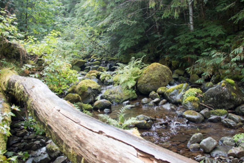
Gary and Natalia decided to work together to explore PFAS in Biscayne Bay. This area is a crucial estuary around Miami, providing a unique environment that supports diverse wildlife and local industries. As a young person, Gary would go shrimping along the bay. He really enjoyed the natural beauty of such a precious resource right in his backyard. Unfortunately, today, Biscayne Bay faces numerous
environmental challenges.
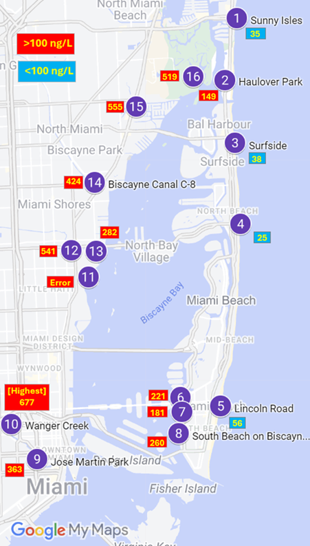
One challenge is PFAS, which enters the estuary through water pollution that drains into the bay. Gary expected PFAS to be highest in the urban freshwater streams that drain into the bay because human activity is high, and a lot of chemicals are released into the water. He thought that the bay would also have high concentrations of PFAS because the streams drain into the bay, but the surrounding land limits the water from mixing with the ocean. Once the water makes it to the ocean, the chemicals should be able to mix with the larger body of water, lowering the concentration of PFAS.
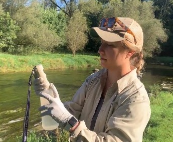
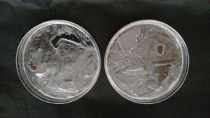
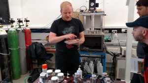
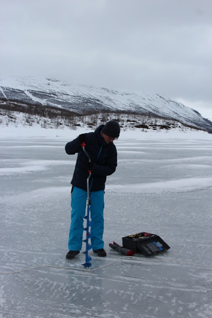
Gary and Natalia identified 16 water sampling sites in water bodies near Miami. They broke these sites into three categories: (1) freshwater rivers that bring water from urban areas into the bay, (2) brackish water, which means a mixture of freshwater and saltwater, located within Biscayne Bay, and (3) salt water found in the Atlantic Ocean. Courtney, a graduate student in Natalia’s lab, joined the team to assist Gary with collecting data and using the technical instruments needed to analyze the samples. Together, they collected one 500 mL sample from each site. To ensure accuracy in the collection of data, they collected two samples from the South Beach pump station site. Gary and Natalia brought the samples back to the lab and ran the samples through instruments that measured PFAS levels. Gary predicted that he would find high levels of PFAS in the freshwater canals and the brackish water of Biscayne Bay, but less in the open ocean.
Featured scientists: Gary Yoham from Miami Senior High School with Natalia Soares Quinete and Courtney Heath from Florida International University