The activities are as follows:
Most people use fossil fuels like natural gas, coal, and oil daily. We use them to generate much of the energy that gets us from place to place, power our homes, and more. Fossil fuels are very efficient at producing energy, but they also come with negative consequences. For example, when burned, they release greenhouse gases like carbon dioxide into our atmosphere. The right balance of greenhouse gasses is needed to keep our planet warm enough to live on. However, because we have burned so many fossil fuels, the earth has gotten too hot too fast, resulting in climate change. Scientists are looking for other ways to fuel our lives with less damage to our environment.
Substituting fossil fuels with biofuels is one of these options. Biofuels are fuels made from plants. Unlike fossil fuels, which take millions of years to form, biofuels are renewable. They are made from plants grown and harvested every few years. Using biofuels instead of fossil fuels can be better for our environment because they do not release ancient carbon like burning fossil fuels does. In addition, the plants made into biofuels take in carbon dioxide from the atmosphere as they grow.
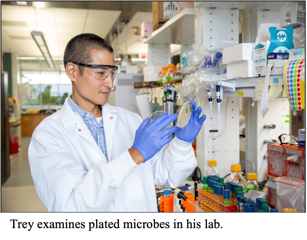
To become biofuels, plants need to go through a series of chemical and physical processes. The sugar stored in plant cells must undergo fermentation. In this process, microorganisms, like yeast, transform the sugars into ethanol that can be used for fuels. Trey is a scientist at the Great Lakes Bioenergy Center. He is interested in seeing how yeast’s ability to transform sugar into fuel is affected by environmental conditions in fields, such as temperature and rainfall.
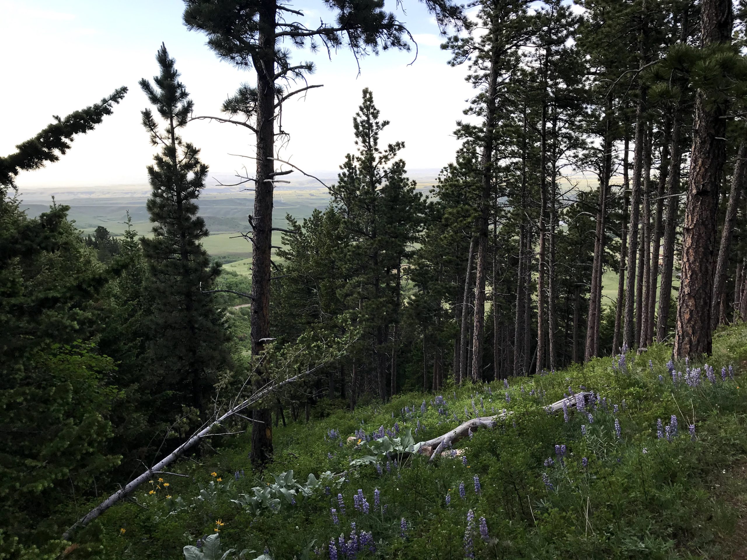
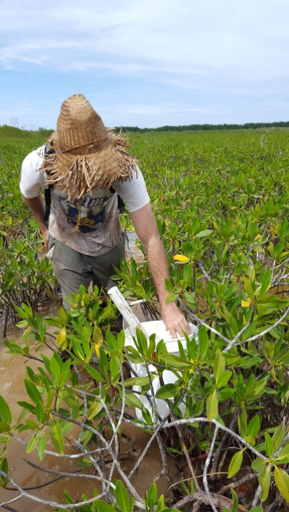
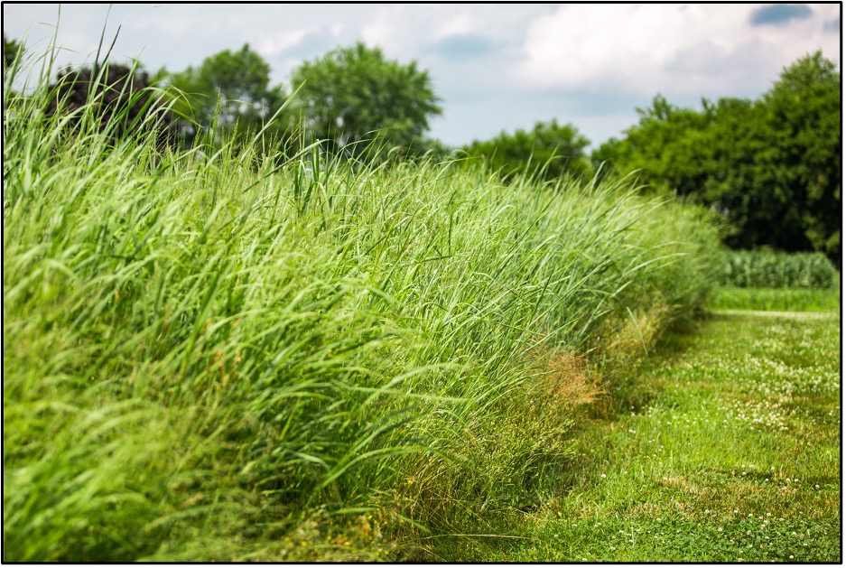
When there was a major drought in 2012, Trey used the opportunity to study the impacts of drought. The growing season had very high temperatures and very low rainfall. These conditions make it more difficult for plants to grow, including switchgrass, a prairie grass being studied as a potential biofuel source.
Trey knew that drought affects the amount and quality of switchgrass that can be harvested. He wanted to find out if drought also had effects on the ability of yeast to transform the plants’ sugars into ethanol. Stress from droughts is known to cause a build-up of compounds in plant cells that help them survive during drought. Trey thought that these extra compounds might harm the yeast or make it difficult for the yeast to break down the sugars during the fermentation process. Trey and his team predicted that if they fed yeast a sample of switchgrass grown during the 2012 drought, the yeast would struggle to ferment its sugars and produce fewer biofuels as a result.
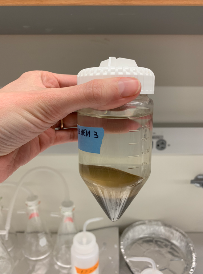
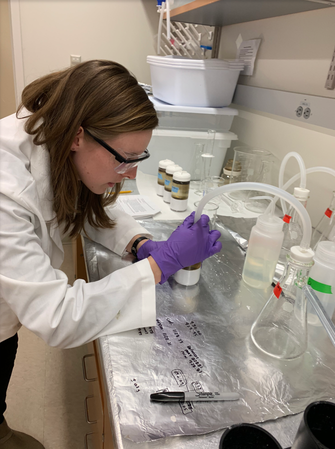
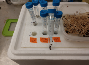
To test their idea, the team studied two different sets of switchgrass samples that were grown and collected in Wisconsin. One set of switchgrass was grown in 2010 under normal conditions. The other set was grown during the 2012 drought. The team introduced the two samples to yeast in a controlled setting and performed four fermentation tests for each set of switchgrass. They recorded the amount of ethanol produced during each test.
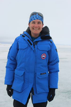
Featured scientists: Trey Sato from the University of Wisconsin-Madison. Written by Marina Kerekes.
Flesch–Kincaid Reading Grade Level = 8.2
Additional teacher resources related to this Data Nugget include:
There are other Data Nuggets that share biofuels research. Search this table for “GLBRC” to find more! Some of the popular activities include:
The Great Lakes Bioenergy Research Center (GLBRC) has many biofuel-related resources available to K16 educators on their webpage.
For activities related specifically to this Data Nugget, see:
- Fermentation in a Bag (elementary – high school level)
- CB2E: Converting Cellulosic Biomass to Ethanol (high school – undergraduate level)